Booking.com European landscape analysis
Importing the Data Set
Story Time
As a team member of Data Analytics Team at Booking.com, I have been asked to gather insights on the mid- to high-end (luxury) hotel market in Europe. I am to present my results to my Team Lead.
#`## Cleaning Data Set global_hotel_chain_sizec
First, let’s have a look at the overall global luxury & upscale hotel market.
# let's have a look on our data set
#describe(global_hotel_chain_size)
#Remove empty columns and rows
global_hotel_chain_size_clean<-remove_empty(global_hotel_chain_size, which = c("rows","cols"))
#describe(global_hotel_chain_size_clean)
Cleaning Data Set hotels_raw
glimpse(hotels_raw)## Rows: 515,738
## Columns: 17
## $ hotel_address <chr> "s Gravesandestraat 55 Oos…
## $ additional_number_of_scoring <dbl> 194, 194, 194, 194, 194, 1…
## $ review_date <chr> "8/3/2017", "8/3/2017", "7…
## $ average_score <dbl> 7.7, 7.7, 7.7, 7.7, 7.7, 7…
## $ hotel_name <chr> "Hotel Arena", "Hotel Aren…
## $ reviewer_nationality <chr> "Russia", "Ireland", "Aust…
## $ negative_review <chr> "I am so angry that i made…
## $ review_total_negative_word_counts <dbl> 397, 0, 42, 210, 140, 17, …
## $ total_number_of_reviews <dbl> 1403, 1403, 1403, 1403, 14…
## $ positive_review <chr> "Only the park outside of …
## $ review_total_positive_word_counts <dbl> 11, 105, 21, 26, 8, 20, 18…
## $ total_number_of_reviews_reviewer_has_given <dbl> 7, 7, 9, 1, 3, 1, 6, 1, 3,…
## $ reviewer_score <dbl> 2.9, 7.5, 7.1, 3.8, 6.7, 6…
## $ tags <chr> "[' Leisure trip ', ' Coup…
## $ days_since_review <chr> "0 days", "0 days", "3 day…
## $ lat <dbl> 52.4, 52.4, 52.4, 52.4, 52…
## $ lng <dbl> 4.92, 4.92, 4.92, 4.92, 4.…hotels_date_correct<-hotels_raw %>% mutate(review_date=as.Date(review_date,"%d/%m/%Y")) %>% mutate(country=word(hotel_address,-1,sep=fixed(" ")))
#glimpse(hotels_date_correct)#Remove empty columns and rows
hotel1<-remove_empty(hotels_date_correct, which = c("rows","cols"))%>%
filter(!is.na(lat))
#Check for duplicates (visualize bots)
duplicates<-hotel1%>%get_dupes(positive_review, negative_review, hotel_name, reviewer_nationality)
#duplicates
#delete duplicates
hotel2<-hotel1%>%
distinct(positive_review, negative_review, hotel_name, reviewer_nationality, .keep_all = TRUE)
md.pattern(hotel2,rotate.names = T)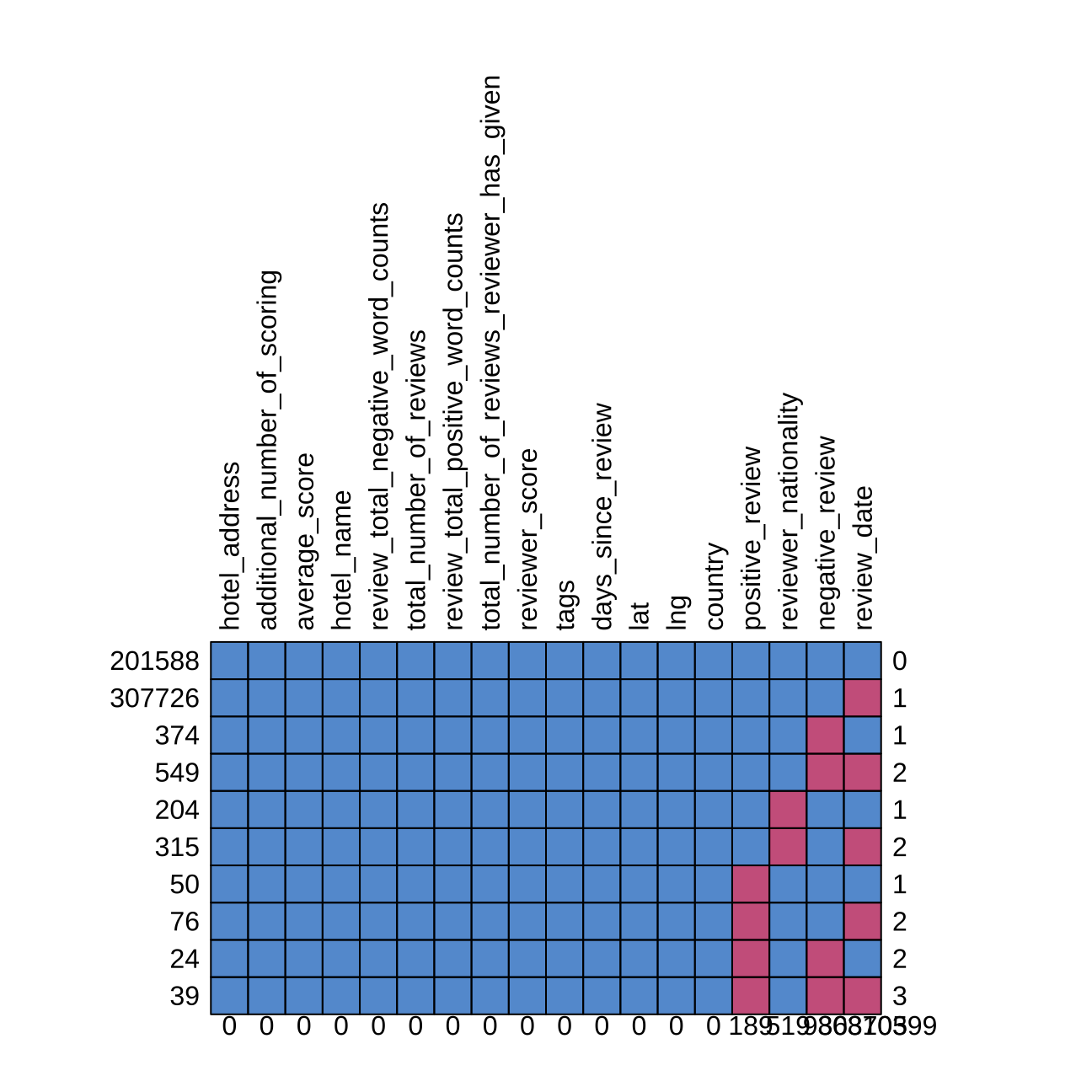
##        hotel_address additional_number_of_scoring average_score hotel_name
## 201588             1                            1             1          1
## 307726             1                            1             1          1
## 374                1                            1             1          1
## 549                1                            1             1          1
## 204                1                            1             1          1
## 315                1                            1             1          1
## 50                 1                            1             1          1
## 76                 1                            1             1          1
## 24                 1                            1             1          1
## 39                 1                            1             1          1
##                    0                            0             0          0
##        review_total_negative_word_counts total_number_of_reviews
## 201588                                 1                       1
## 307726                                 1                       1
## 374                                    1                       1
## 549                                    1                       1
## 204                                    1                       1
## 315                                    1                       1
## 50                                     1                       1
## 76                                     1                       1
## 24                                     1                       1
## 39                                     1                       1
##                                        0                       0
##        review_total_positive_word_counts
## 201588                                 1
## 307726                                 1
## 374                                    1
## 549                                    1
## 204                                    1
## 315                                    1
## 50                                     1
## 76                                     1
## 24                                     1
## 39                                     1
##                                        0
##        total_number_of_reviews_reviewer_has_given reviewer_score tags
## 201588                                          1              1    1
## 307726                                          1              1    1
## 374                                             1              1    1
## 549                                             1              1    1
## 204                                             1              1    1
## 315                                             1              1    1
## 50                                              1              1    1
## 76                                              1              1    1
## 24                                              1              1    1
## 39                                              1              1    1
##                                                 0              0    0
##        days_since_review lat lng country positive_review reviewer_nationality
## 201588                 1   1   1       1               1                    1
## 307726                 1   1   1       1               1                    1
## 374                    1   1   1       1               1                    1
## 549                    1   1   1       1               1                    1
## 204                    1   1   1       1               1                    0
## 315                    1   1   1       1               1                    0
## 50                     1   1   1       1               0                    1
## 76                     1   1   1       1               0                    1
## 24                     1   1   1       1               0                    1
## 39                     1   1   1       1               0                    1
##                        0   0   0       0             189                  519
##        negative_review review_date
## 201588               1           1      0
## 307726               1           0      1
## 374                  0           1      1
## 549                  0           0      2
## 204                  1           1      1
## 315                  1           0      2
## 50                   1           1      1
## 76                   1           0      2
## 24                   0           1      2
## 39                   0           0      3
##                    986      308705 310399
Europe vs. different continents - Luxury Chains, Upper Upscale Chains
Now I am good to go.
First analysis:
 # distribution of all the variables chain scale
data.frame(table(global_hotel_chain_size_clean$chain_scale))
## Var1 Freq
## 1 Economy Chains 141
## 2 Luxury Chains 115
## 3 Midscale Chains 174
## 4 Upper Midscale Chains 225
## 5 Upper Upscale Chains 161
## 6 Upscale Chains 276# changing variables to factors
global_hotel_chain_size_clean$chain_scale <- global_hotel_chain_size_clean$chain_scale %>% factor(levels= c("Economy Chains", "Midscale Chains", "Upper Midscale Chains","Upscale Chains", "Upper Upscale Chains", "Luxury Chains" ))
# checking if the data is correct
data.frame(table(global_hotel_chain_size_clean$chain_scale))## Var1 Freq
## 1 Economy Chains 141
## 2 Midscale Chains 174
## 3 Upper Midscale Chains 225
## 4 Upscale Chains 276
## 5 Upper Upscale Chains 161
## 6 Luxury Chains 115# pivoting the data & cleaning
chain_size_pivot<-global_hotel_chain_size_clean %>%
pivot_longer(cols = 5:11, names_to= "region", values_to= "x", values_drop_na = TRUE) %>%
mutate( region = case_when(
region== "africa" ~ "Africa",
region=="apac" ~ "APAC countries",
region== "c_s_america" ~ "Central & South America",
region== "europe" ~ "Europe",
region== "middle_east" ~ "Middle East",
region== "n_america_excl_us" ~ "North America exlc. US",
region== "united_states" ~ "United States",
)) %>%
select(-x)
# Luxury Chains across countries
chain_size_pivot_relevant<- chain_size_pivot %>%
filter(chain_scale== "Luxury Chains"|| chain_scale== "Upper Upscale Chains" || chain_scale== "Upscale Chains" ) %>%
group_by( region) %>%
summarise(count=n())
# Upper Upscale Chains across countires
chain_size_pivot %>%
filter(chain_scale== "Upper Upscale Chains") %>%
group_by( region) %>%
summarise(count=n())## # A tibble: 7 x 2
## region count
## <chr> <int>
## 1 Africa 33
## 2 APAC countries 78
## 3 Central & South America 29
## 4 Europe 95
## 5 Middle East 34
## 6 North America exlc. US 30
## 7 United States 57#Upscale Chains across countires
chain_size_pivot %>%
filter(chain_scale== "Upscale Chains") %>%
group_by( region) %>%
summarise(count=n())## # A tibble: 7 x 2
## region count
## <chr> <int>
## 1 Africa 33
## 2 APAC countries 110
## 3 Central & South America 40
## 4 Europe 153
## 5 Middle East 37
## 6 North America exlc. US 43
## 7 United States 56# charts showing how big Europe is in these sectors
my_colours <- c("grey70", "#2FABE1")
is_europe<- chain_size_pivot_relevant%>%
mutate(
is_europe = ifelse(region == "Europe", TRUE, FALSE))
# Chart of the data across all the regions
first_plot<- ggplot(is_europe, aes(x=reorder(region,-count), y=count, fill=is_europe)) +
geom_bar(stat="identity", alpha=0.8)+
theme_minimal() +
theme(panel.grid.major.y = element_line(color = "gray60", size = 0.1),
panel.background = element_rect(fill = "white", colour = "white"),
axis.line = element_line(size = 1, colour = "grey80"),
axis.ticks = element_line(size = 3,colour = "grey80"),
axis.ticks.length = unit(.20, "cm"),
plot.title = element_text(color = "#043680",size=15,face="bold", family= "Montserrat"),
plot.subtitle = element_text(color = "#043680", face="bold", ,size= 10,family= "Montserrat"),
plot.caption = element_text(color = "grey40", face="italic", ,size= 7,family= "Montserrat",hjust=0),
axis.title.y = element_text(size = 8, angle = 90, family="Montserrat", face = "bold"),
axis.text.y=element_text(family="Montserrat", size=7),
axis.title.x = element_text(size = 8, family="Montserrat", face = "bold"),
axis.text.x=element_text(family="Montserrat", size=7),
legend.text=element_text(family="Montserrat", size=7),
legend.title=element_text(family="Montserrat", size=8, face="bold"),
legend.position = "none")+
labs(title = " Europe is the most aboundant region \nin Luxury & Upper Upscale Chains", subtitle= "Number of Luxury, Upper Upscale & Upscale Chains across the regions", x="Region", y=" Number of chians", caption="Source: https://www.kaggle.com/ployyyywa/global-hotel-chain-presence") +
scale_y_continuous()+
scale_fill_manual(values = my_colours)+
geom_label(aes(label=count),family = "Montserrat", fontface="bold", color="grey20", )
first_plot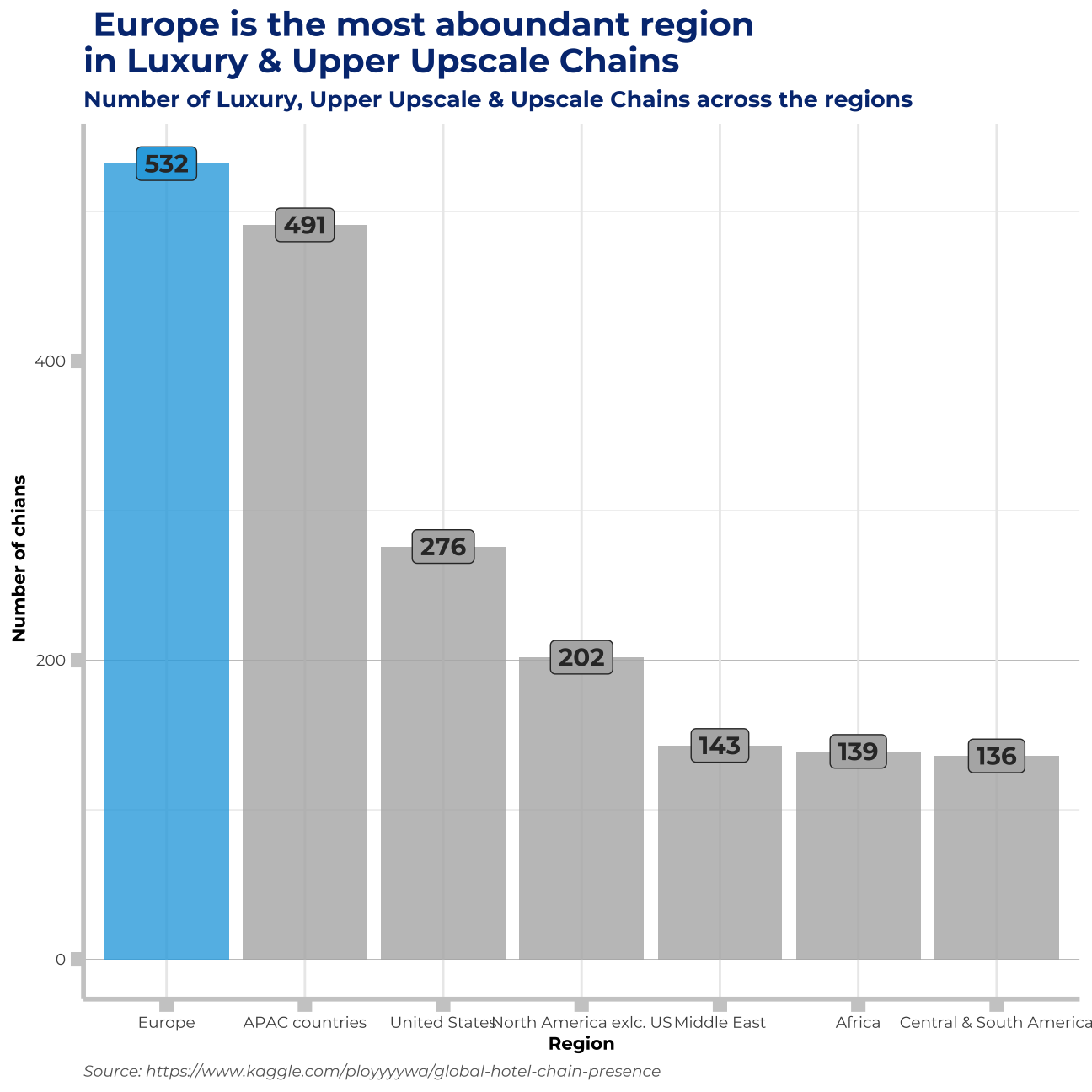
European landscape in terms of chain types
# data on how in Europe the chains are distributed
chain_types_europe<- chain_size_pivot %>%
  filter(region=="Europe") %>%
  group_by( chain_scale) %>%
  summarise(count=n())
my_colours2 <- c("grey70", "#043680")
is_chain<-  chain_types_europe%>%
mutate(
    is_chain = ifelse(chain_scale == "Luxury Chains",  TRUE,
                      ifelse(chain_scale== "Upper Upscale Chains", TRUE, FALSE)))
# Chart of the data across all the regions
  my_text <- "Upper Upscale + Luxury = 162"

ggplot(is_chain, aes(x=reorder(chain_scale,chain_scale), y=count, fill=is_chain)) +
    geom_bar(stat="identity", alpha=0.8)+
theme_minimal() +
  theme(panel.grid.major.y = element_line(color = "gray60", size = 0.1),
        panel.background = element_rect(fill = "white", colour = "white"),
        axis.line = element_line(size = 1, colour = "grey80"),
        axis.ticks = element_line(size = 3,colour = "grey80"),
        axis.ticks.length = unit(.20, "cm"),
        plot.title = element_text(color = "#2FABE1",size=15,face="bold", family= "Montserrat"),
        plot.subtitle = element_text(color = "#2FABE1", face="bold", ,size= 10,family= "Montserrat"),
        plot.caption = element_text(color = "grey40", face="italic", ,size= 7,family= "Montserrat",hjust=0),
        axis.title.y = element_text(size = 8, angle = 90, family="Montserrat", face = "bold"),
        axis.text.y=element_text(family="Montserrat", size=7),
        axis.title.x = element_text(size = 8, family="Montserrat", face = "bold"),
        axis.text.x=element_text(family="Montserrat", size=7),
        legend.text=element_text(family="Montserrat", size=7),
        legend.title=element_text(family="Montserrat", size=8, face="bold"),
        legend.position = "none")+
    labs(title = "Europe seems to be abundant in the chains of our aim ", subtitle= "Number of all the types of chains in Europe", x="Hotel sector", y=" Number of chians", caption="Source: https://www.kaggle.com/ployyyywa/global-hotel-chain-presence") +
  scale_y_continuous()+
  scale_fill_manual(values = my_colours2)+
   geom_label(aes(label=count),family = "Montserrat", fontface="bold", color="white", )+
   annotate(geom= "text", x=5.5,  y=110, label=my_text, family="Montserrat",size=5, color="#2FABE1", fontface="bold")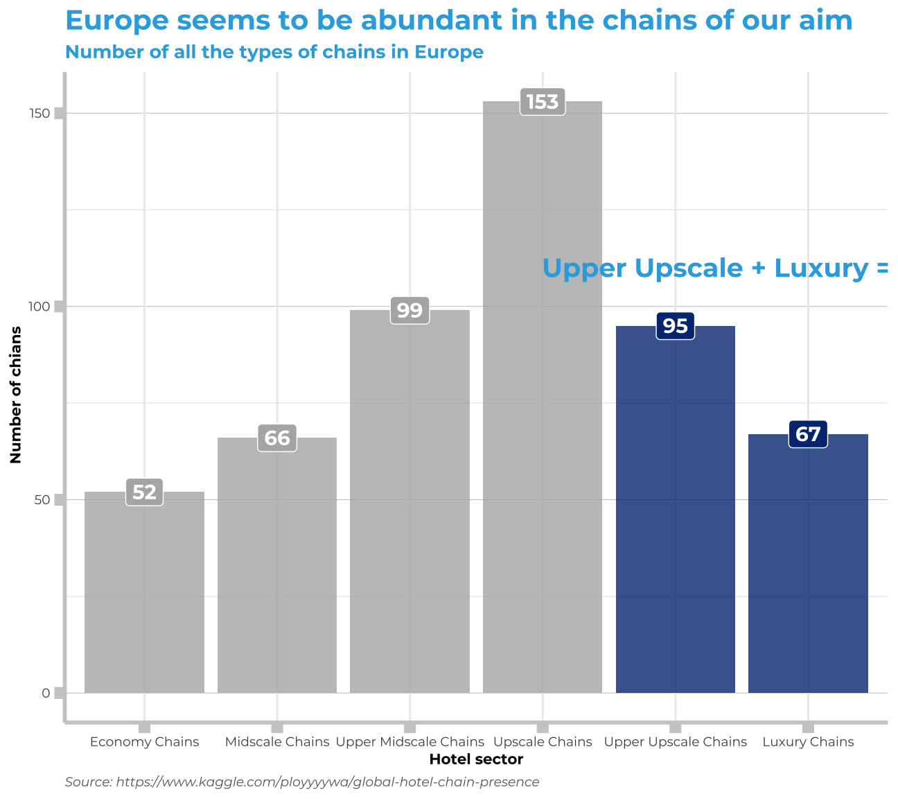
Average rating of hotels by country
#7.hotels with highest ratings (possible: combined with location)
#average rating of hotels by country
hotel3<-hotel2 %>%
  distinct(hotel_name,average_score,country)%>%
  select(country,average_score)

my_colours3 <- c("white", "#2FABE1")
is_france<-  hotel3%>%
mutate(
    is_france = ifelse(country == "France",  TRUE, FALSE)) %>%
   mutate(country=recode(country, "Kingdom" = "United Kingdom"))
ggplot(is_france, aes(x=average_score,y=reorder(country,average_score),fill=is_france))+
  geom_violin()+
  geom_boxplot(width=0.1)+
  theme_minimal() +
  theme(panel.grid.major.y = element_line(color = "gray60", size = 0.1),
        panel.background = element_rect(fill = "white", colour = "white"),
        axis.line = element_line(size = 1, colour = "grey80"),
        axis.ticks = element_line(size = 3,colour = "grey80"),
        axis.ticks.length = unit(.20, "cm"),
        plot.title = element_text(color = "black",size=15,face="bold", family= "Montserrat"),
        plot.subtitle = element_text(color = "#043680", face="bold", ,size= 10,family= "Montserrat"),
        plot.caption = element_text(color = "grey40", face="italic", ,size= 7,family= "Montserrat",hjust=0),
        axis.title.y = element_text(size = 8, angle = 90, family="Montserrat", face = "plain"),
        axis.text.y=element_text(family="Montserrat", size=7),
        axis.title.x = element_text(size = 8, family="Montserrat", face = "plain"),
        axis.text.x=element_text(family="Montserrat", size=7),
        legend.text=element_text(family="Montserrat", size=7),
        legend.title=element_text(family="Montserrat", size=8, face="bold"),
        legend.position = "none")+
    labs(title = "France has the highest median rating", subtitle= "Distribution of average ratings of hotels across 6 selected countries", x="Average rating of hotels", y="Country", caption="Source: https://www.kaggle.com/ployyyywa/global-hotel-chain-presence") +
  scale_fill_manual(values = my_colours3)
Hotels of excellent ratings, by country
##hotels with highest ratings
##choose all hotels > 8/8.5/9
hotel4<-hotel3%>%
  filter(average_score>=9)%>%
  group_by(country)%>%
  summarise(count=n())%>%
  mutate(is_best=ifelse(country=="Kingdom"|country=="France",1,0))
ggplot(hotel4,aes(x=reorder(country,count),y=count,fill=factor(is_best)))+
  geom_col(position="dodge")+
  theme_minimal() +
  theme(panel.grid.major.y = element_line(color = "gray60", size = 0.1),
        panel.background = element_rect(fill = "white", colour = "white"),
        axis.line = element_line(size = 1, colour = "grey80"),
        axis.ticks = element_line(size = 3,colour = "grey80"),
        axis.ticks.length = unit(.20, "cm"),
        plot.title = element_text(color = "black",size=15,face="bold", family= "Montserrat"),
        plot.subtitle = element_text(color = "#043680", face="bold", ,size= 10,family= "Montserrat"),
        plot.caption = element_text(color = "grey40", face="italic", ,size= 7,family= "Montserrat",hjust=0),
        axis.title.y = element_text(size = 8, angle = 90, family="Montserrat", face = "plain"),
        axis.text.y=element_text(family="Montserrat", size=7),
        axis.title.x = element_text(size = 8, family="Montserrat", face = "plain"),
        axis.text.x=element_text(family="Montserrat", size=7, angle=30, hjust=1),
        legend.text=element_text(family="Montserrat", size=7),
        legend.title=element_text(family="Montserrat", size=8, face="bold"),
        legend.position="none")+
    labs(title = "UK & France dominate hotels with >9 average rating", subtitle= "Number of >9 rating hotels in 6 selected countries", x="Country", y="No. of hotels with rating >9", caption="Source: https://www.kaggle.com/ployyyywa/global-hotel-chain-presence")+
  scale_fill_manual(values=c("grey80","#2FABE1")) +
  coord_flip()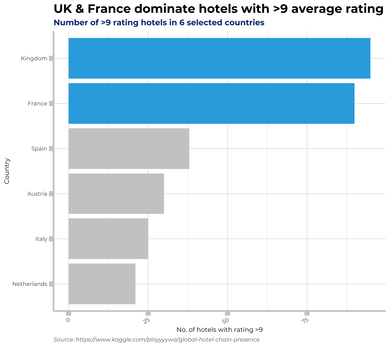
Proportion of Top 5 Reviewer Nationalities per Country
maggiehoteldata <- hotel2 %>% mutate(country=recode(
  country, `Kingdom`= "United Kingdom")) %>%  # change Kingdom to United Kingdom to allow matching
  rename(hotelcountry = country)
# UK
## get counts and proportions of reviewer nationalities
ukdata <- maggiehoteldata %>%
  filter(hotelcountry == "United Kingdom") %>%
  group_by(reviewer_nationality) %>%
  summarise(countreviewernat = n(),
            propreviewernat = countreviewernat / 261509) %>%
  arrange(desc(countreviewernat)) %>%
  mutate(hotelcountry = "United Kingdom") %>%
  slice(1:5)
# ukdata %>%
  # summarise(sumcount = sum(countreviewernat))
# 261509 total reviews
# Netherlands
## get counts and proportions of reviewer nationalities
nldata <- maggiehoteldata %>%
  filter(hotelcountry == "Netherlands") %>%
  group_by(reviewer_nationality) %>%
  summarise(countreviewernat = n(),
            propreviewernat = countreviewernat / 57119) %>%
  arrange(desc(countreviewernat)) %>%
  mutate(hotelcountry = "Netherlands") %>%
  slice(1:5)
# nldata %>%
  # summarise(sumcount = sum(countreviewernat))
# 57119 total reviews
# Austria
## get counts and proportions of reviewer nationalities
ausdata <- maggiehoteldata %>%
  filter(hotelcountry == "Austria") %>%
  group_by(reviewer_nationality) %>%
  summarise(countreviewernat = n(),
            propreviewernat = countreviewernat / 36241) %>%
  arrange(desc(countreviewernat)) %>%
  mutate(hotelcountry = "Austria") %>%
  slice(1:5)
# ausdata %>%
 #  summarise(sumcount = sum(countreviewernat))
# 36241 total reviews
# Spain
## get counts and proportions of reviewer nationalities
spaindata <- maggiehoteldata %>%
  filter(hotelcountry == "Spain") %>%
  group_by(reviewer_nationality) %>%
  summarise(countreviewernat = n(),
            propreviewernat = countreviewernat / 59895) %>%
  arrange(desc(countreviewernat)) %>%
  mutate(hotelcountry = "Spain") %>%
  slice(1:5)
 # spaindata %>%
   # summarise(sumcount = sum(countreviewernat))
# 59895 total reviews
# France
## get counts and proportions of reviewer nationalities
francedata <- maggiehoteldata %>%
  filter(hotelcountry == "France") %>%
  group_by(reviewer_nationality) %>%
  summarise(countreviewernat = n(),
            propreviewernat = countreviewernat / 59011 ) %>%
  arrange(desc(countreviewernat)) %>%
  mutate(hotelcountry = "France") %>%
  slice(1:5)
# francedata %>%
   # summarise(sumcount = sum(countreviewernat))
# 59011  total reviews
# Italy
## get counts and proportions of reviewer nationalities
italydata <- maggiehoteldata %>%
  filter(hotelcountry == "Italy") %>%
  group_by(reviewer_nationality) %>%
  summarise(countreviewernat = n(),
            propreviewernat = countreviewernat / 37170) %>%
  arrange(desc(countreviewernat)) %>%
  mutate(hotelcountry = "Italy") %>%
  slice(1:5)
# italydata %>%
   # summarise(sumcount = sum(countreviewernat))
# 37170 total reviews
# Combine all of the above
top5reviewernat <- rbind(ukdata,
                         nldata,
                         spaindata,
                         francedata,
                         italydata,
                         ausdata)
 countrylevels <- names(sort(tapply(top5reviewernat$propreviewernat, # create levels to have stacked bar chart according to size not alphabetical order
                                    top5reviewernat$reviewer_nationality,
                                    sum)))
# Code for barplot

stackedbarplot <- ggplot(top5reviewernat, aes(x = hotelcountry, y = propreviewernat,
                            fill = factor(reviewer_nationality, levels = countrylevels))) +
  geom_bar(stat = "identity") +
  scale_fill_manual(values = c("#810f7c", "#8856a7", "#8c96c6", "#9ebcda", "#bfd3e6", "#edf8fb",
                              "#ccebc5", "#a8ddb5", "#7bccc4", "#43a2ca", "#0868ac", "darkblue")) +
  labs(title = "Brits take over as Majority Reviewers",
       subtitle = "Proportion of Top 5 Reviewer Nationalities per Country",
      y = "Proportion of Total Reviews",
      x = " ") +
  theme(legend.title = element_blank(),
panel.grid.major.y = element_line(color = "gray60", size = 0.1),
        panel.background = element_rect(fill = "white", colour = "white"),
        axis.line = element_line(size = 1, colour = "grey80"),
        axis.ticks = element_line(size = 3,colour = "grey80"),
        plot.title = element_text(size=15,face="bold", family= "Montserrat"),
        plot.subtitle = element_text(face="plain", ,size= 10,family= "Montserrat"),
        plot.caption = element_text(color = "grey40", face="italic", ,size= 7,family= "Montserrat",hjust=0),
        axis.title.y = element_text(size = 8, angle = 90, family="Montserrat", face = "bold"),
        axis.text.y=element_text(family="Montserrat", size=7),
        axis.title.x = element_text(size = 8, family="Montserrat", face = "bold"),
        axis.text.x=element_text(family="Montserrat", size=7),
        legend.text=element_text(family="Montserrat", size=7))

stackedbarplot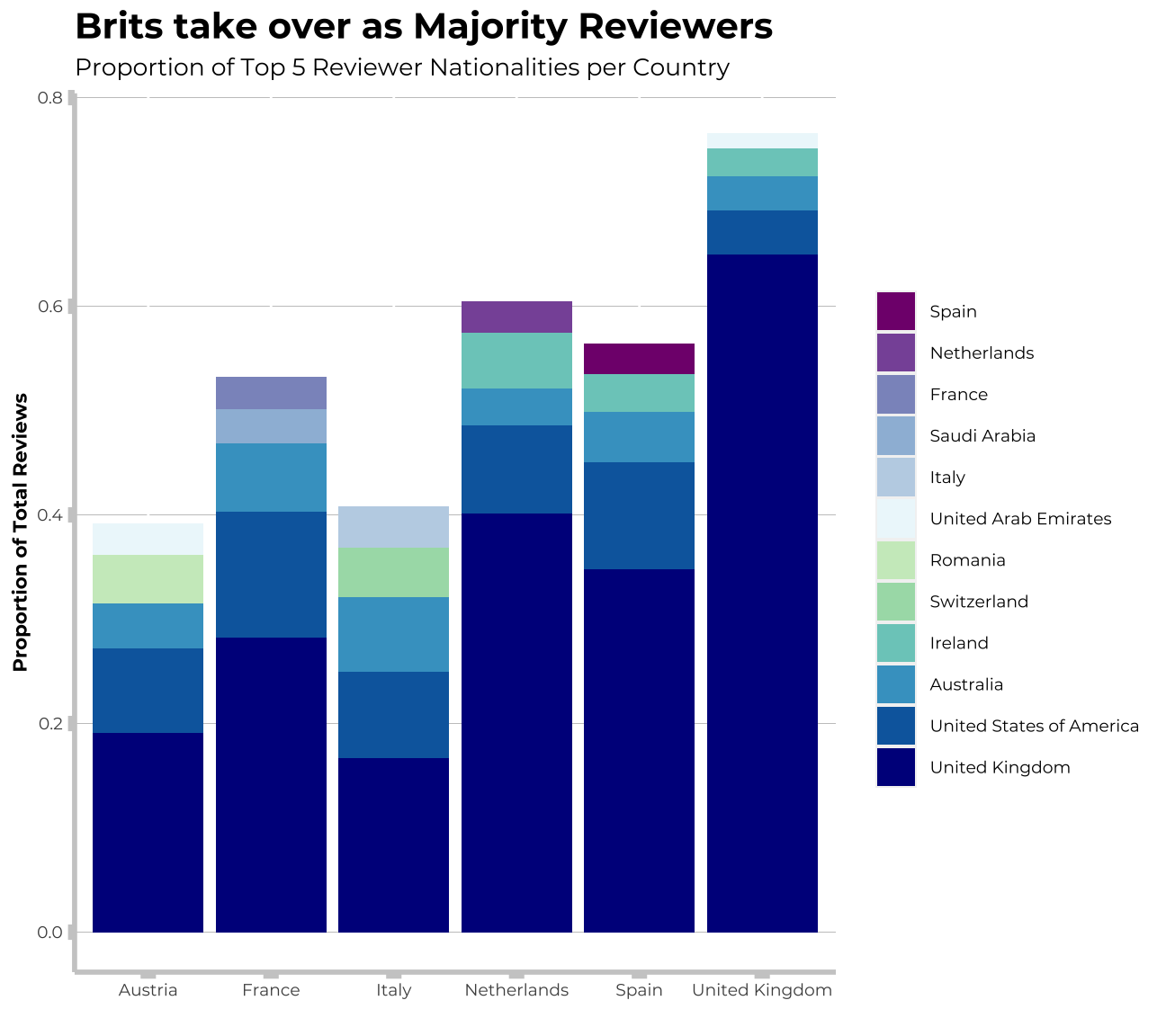
Region and subregion reviers’ background
Creating variables
glimpse(hotel2)## Rows: 510,945
## Columns: 18
## $ hotel_address <chr> "s Gravesandestraat 55 Oos…
## $ additional_number_of_scoring <dbl> 194, 194, 194, 194, 194, 1…
## $ review_date <date> 2017-03-08, 2017-03-08, N…
## $ average_score <dbl> 7.7, 7.7, 7.7, 7.7, 7.7, 7…
## $ hotel_name <chr> "Hotel Arena", "Hotel Aren…
## $ reviewer_nationality <chr> "Russia", "Ireland", "Aust…
## $ negative_review <chr> "I am so angry that i made…
## $ review_total_negative_word_counts <dbl> 397, 0, 42, 210, 140, 17, …
## $ total_number_of_reviews <dbl> 1403, 1403, 1403, 1403, 14…
## $ positive_review <chr> "Only the park outside of …
## $ review_total_positive_word_counts <dbl> 11, 105, 21, 26, 8, 20, 18…
## $ total_number_of_reviews_reviewer_has_given <dbl> 7, 7, 9, 1, 3, 1, 6, 1, 3,…
## $ reviewer_score <dbl> 2.9, 7.5, 7.1, 3.8, 6.7, 6…
## $ tags <chr> "[' Leisure trip ', ' Coup…
## $ days_since_review <chr> "0 days", "0 days", "3 day…
## $ lat <dbl> 52.4, 52.4, 52.4, 52.4, 52…
## $ lng <dbl> 4.92, 4.92, 4.92, 4.92, 4.…
## $ country <chr> "Netherlands", "Netherland…hotel_review_nationality<- hotel2 %>% #merging main table with countries and continents of reviwers' origin
left_join(country_continent, by=c("reviewer_nationality"="name")) %>%
drop_na(reviewer_nationality, region)
reviews_by_region<- hotel_review_nationality %>% #creating summary for regions
group_by(region) %>%
summarise(avg_review= mean(reviewer_score),
avg_no_positive= mean(review_total_positive_word_counts),
avg_no_negative= mean(review_total_negative_word_counts)) %>%
arrange(desc(avg_review))
reviews_by_subregion<- hotel_review_nationality %>% #creating summary for subregions
group_by(region,sub_region) %>%
summarise(avg_review= mean(reviewer_score),
avg_no_positive= mean(review_total_positive_word_counts),
avg_no_negative= mean(review_total_negative_word_counts)) %>%
arrange(desc(avg_review))Reviewers’ origin by region
# pivoting regions
reviews_by_region_pivot<- reviews_by_region %>%
  pivot_longer(cols = 3:4, names_to= "type_review", values_to= "score", values_drop_na = TRUE) # pivoted dataframe
reviews_by_region_pivot$type_review<- reviews_by_region_pivot$type_review %>%  factor(levels= c("avg_no_negative", "avg_no_positive")) # creating avg no of positive & negative words per region + average review score per region
# creating a cool chart
reviews_by_region_pivot <- reviews_by_region_pivot%>%
  mutate(score_chart = ifelse(type_review == "avg_no_positive",
                                 score,
                                 -1*score)) %>%
  mutate(is_extreme = ifelse(score_chart>20, "1",
                             ifelse(score_chart< -19, "2",
                                    ifelse(score_chart>-19 & score_chart <0, "3", "4"))))

my_colours_positive<- c("#45B05F", "tomato","#FFBAAD","#A8DDB5") # scale for the chart

  my_text1r <- "Negative"
    my_text2r <- "Positive"
    my_text3r <- "Average review score"

# negative and positive
reviews_by_region_pivot %>%
  ggplot(aes(x = reorder(region,avg_review), fill=is_extreme))+
  geom_bar(aes(y = score_chart),stat = "identity")+
  coord_flip() +
  theme_minimal()+
  geom_text(aes(y=avg_review, label=round(avg_review,1)),family = "Montserrat", fontface="bold", colour="black")+
  scale_y_continuous(breaks=seq(-20,20,5)) +
  theme(panel.grid.major.y = element_line(color = "gray60", size = 0.1),
        panel.background = element_rect(fill = "white", colour = "white"),
        axis.line = element_line(size = 1, colour = "grey80"),
        axis.ticks = element_line(size = 3,colour = "grey80"),
        axis.ticks.length = unit(.20, "cm"),
        plot.title = element_text(color = "grey20",size=15,face="bold", family= "Montserrat"),
        plot.subtitle = element_text(color = "grey40", face="plain",size= 10,family= "Montserrat"),
        plot.caption = element_text(color = "grey40", face="italic",size= 7,family= "Montserrat",hjust=0),
        axis.title.y = element_text(size = 8, angle = 90, family="Montserrat", face = "bold"),
        axis.text.y=element_text(family="Montserrat", size=7),
        axis.title.x = element_text(size = 8, family="Montserrat", face = "bold"),
        axis.text.x=element_text(family="Montserrat", size=7),
        legend.text=element_text(family="Montserrat", size=7),
        legend.title=element_text(family="Montserrat", size=8, face="bold"),
        legend.position = "none")+
    labs(title = "The most criticising guests come from Europe,\nthe most positive come from Australia", subtitle= "Number of positive and negative words per review per continent and average review score", x= "Region", y= "Average number of positive/negative words in a review", caption="Source: https://www.kaggle.com/ployyyywa/global-hotel-chain-presence") +
  scale_fill_manual(values = my_colours_positive) +
  scale_y_continuous(labels=abs)+
   geom_hline(yintercept = -18, linetype="dashed",
                color = "tomato", size=0.8)+
  geom_hline(yintercept = 19.5, linetype="dashed",
                color = "#45B05F", size=0.8)+
 annotate(geom= "text", x=5,  y=-2, label=my_text1r, family="Montserrat",size=6, color="tomato", fontface="bold")+
  annotate(geom= "text", x=5,  y=1.9, label=my_text2r, family="Montserrat",size=6, color="#F1FFEB", fontface=2)+
   annotate(geom= "text", x=5.5,  y=9, label=my_text3r, family="Montserrat",size=4, color="black", fontface=2)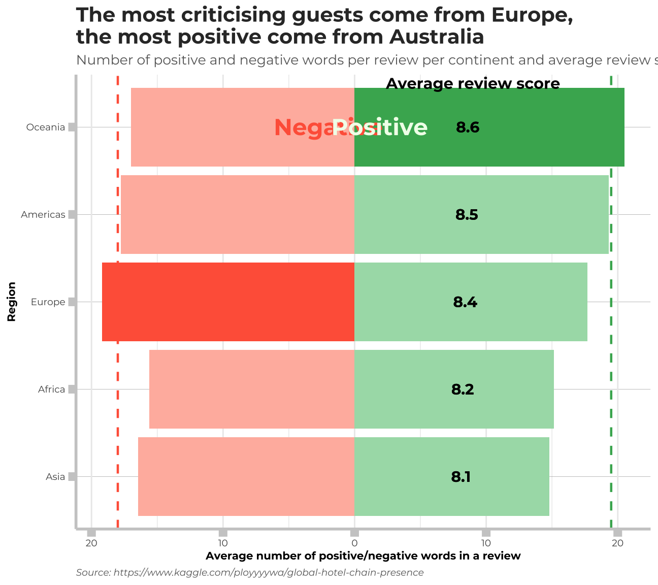
Reviewers’ origin by Subregion
reviews_by_subregion_pivot<- reviews_by_subregion %>%
  pivot_longer(cols = 4:5, names_to= "type_review", values_to= "score", values_drop_na = TRUE) # pivoted dataframe
reviews_by_subregion_pivot$type_review<- reviews_by_subregion_pivot$type_review %>%  factor(levels= c("avg_no_negative", "avg_no_positive")) # creating avg no of positive & negative words per region + average review score per subregion
reviews_by_subregion_pivot <- reviews_by_subregion_pivot%>%
  mutate(score_chart = ifelse(type_review == "avg_no_positive",
                                 score,
                                 -1*score)) %>%
  mutate(is_extreme = ifelse(score_chart>17.5, "1",
                             ifelse(score_chart< -17.5, "2",
                                    ifelse(score_chart>-17.5 & score_chart <0, "3", "4"))))

  my_text1s <- "Negative"
    my_text2s <- "Positive"
    my_text3s <- "Average \nreview score"

reviews_by_subregion_pivot %>%
  ggplot(aes(x = reorder(sub_region,avg_review), fill = is_extreme))+
  geom_bar(aes(y = score_chart),stat = "identity")+
  coord_flip() +
  geom_text(aes(y=avg_review, label=round(avg_review,1)),family = "Montserrat", fontface="bold", colour="black")+
  scale_y_continuous(breaks=seq(-20,20,5)) +
  theme(panel.grid.major.y = element_line(color = "gray60", size = 0.1),
        panel.background = element_rect(fill = "white", colour = "white"),
        axis.line = element_line(size = 1, colour = "grey80"),
        axis.ticks = element_line(size = 3,colour = "grey80"),
        axis.ticks.length = unit(.20, "cm"),
        plot.title = element_text(color = "grey20",size=10,face="bold", family= "Montserrat"),
        plot.subtitle = element_text(color = "grey40", face="plain", ,size= 8,family= "Montserrat"),
        plot.caption = element_text(color = "grey40", face="italic", ,size= 7,family= "Montserrat",hjust=0),
        axis.title.y = element_text(size = 8, angle = 90, family="Montserrat", face = "bold"),
        axis.text.y=element_text(family="Montserrat", size=7),
        axis.title.x = element_text(size = 8, family="Montserrat", face = "bold"),
        axis.text.x=element_text(family="Montserrat", size=7),
        legend.text=element_text(family="Montserrat", size=7),
        legend.title=element_text(family="Montserrat", size=8, face="bold"),
        legend.position = "none")+
    labs(title = "Guests from Europe & North America seem to be \nmost influencial ones and shaping the opinion", subtitle= "Average number of positive/negative words in a review and average review score", x= "Region", y= "Average number of positive/negative words in a review", caption="Source: https://www.kaggle.com/ployyyywa/global-hotel-chain-presence") +
  scale_fill_manual(values = my_colours_positive) +
  scale_y_continuous(labels=abs)+
   geom_hline(yintercept = -17.5, linetype="dashed",
                color = "tomato", size=0.8)+
  geom_hline(yintercept = 17.5, linetype="dashed",
                color = "#45B05F", size=0.8)+
 annotate(geom= "text", x=15,  y=-2, label=my_text1s, family="Montserrat",size=4.5, color="tomato", fontface="bold")+
  annotate(geom= "text", x=15,  y=1.9, label=my_text2s, family="Montserrat",size=4.5, color="#F1FFEB", fontface=2)+
   annotate(geom= "text", x=17,  y=12.5, label=my_text3s, family="Montserrat",size=3.5, color="black", fontface=2)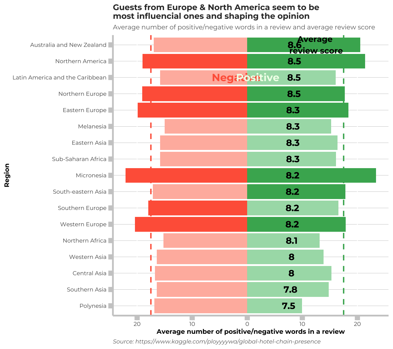
Creating wordclouds with most popular positive/ negative words
Preparing dataset
hotelcloud<-hotel2[!is.na(hotel2$positive_review), ]
hotelcloud<-hotel2[!is.na(hotel2$negative_review), ]
hotelcloud2<-hotelcloud
#clean reviews and select only those with useful information
hotelcloud3<-hotelcloud2 %>%
filter(sapply(strsplit(positive_review, " "), length)>3) %>%
filter(sapply(strsplit(negative_review, " "), length)>3)
#randomly select 6000 data to visualize
hotelcloud4<-hotelcloud3[sample(nrow(hotelcloud3), 6000), ]
rm(hotelcloud3,hotelcloud2)
#build corpus
library(tm)
review_pos <- Corpus(VectorSource(hotelcloud4$positive_review))
review_neg <- Corpus(VectorSource(hotelcloud4$negative_review))
#skip the words: room and hotel, cuz they dont give useful information
words <- c("room","hotel")
review_pos <- tm_map(review_pos, removeWords, words)
review_neg <- tm_map(review_neg, removeWords, words)
#count frequency
DTM_pos <- DocumentTermMatrix(review_pos, control = list(
tolower = TRUE,
removeNumbers = TRUE,
stopwords = TRUE,
removePunctuation = TRUE,
stripWhitespace = TRUE))
dim(DTM_pos) ## [1] 6000 5660DTM_neg <- DocumentTermMatrix(review_neg, control = list(
tolower = TRUE,
removeNumbers = TRUE,
stopwords = TRUE,
removePunctuation = TRUE,
stripWhitespace = TRUE))
inspect(DTM_neg) ## <<DocumentTermMatrix (documents: 6000, terms: 7568)>>
## Non-/sparse entries: 73268/45334732
## Sparsity : 100%
## Maximal term length: 18
## Weighting : term frequency (tf)
## Sample :
## Terms
## Docs bathroom bed bit breakfast didn little one rooms small staff
## 2515 2 1 0 0 0 0 1 0 0 0
## 2620 1 1 0 1 0 1 2 0 0 0
## 292 0 0 0 0 3 0 0 2 0 2
## 3331 0 1 0 3 0 0 1 0 0 0
## 3333 1 4 1 0 2 1 0 0 0 3
## 4033 0 0 1 0 0 0 0 0 0 0
## 4332 0 0 0 0 0 0 2 4 1 0
## 4603 3 0 0 0 2 0 2 0 0 1
## 4721 0 0 1 4 6 0 0 0 0 1
## 5519 0 0 0 1 1 1 0 0 0 2rm(review_neg,review_pos)Positive wordcloud
##Positive wordcloud
#convert to tibble
m <- as.matrix(DTM_pos)
DTM_tbl <- as_tibble(m)
#rm (m,hotel3,DTM_neg,DTM_pos,review_pos,review_neg,DTM_tbl,wordCountDoc_pos)
DTM_pos_tidy <- pivot_longer(DTM_tbl, cols = everything(), names_to = "word", values_to = "wordCount")
# Order by freq
wordCountDoc_pos <- DTM_pos_tidy %>%
        group_by(word) %>%
        summarise(total_pos = sum(wordCount)) %>%
        arrange(desc(total_pos))
print(wordCountDoc_pos %>% top_n(5))
## # A tibble: 5 x 2
## word total_pos
## <chr> <dbl>
## 1 staff 2585
## 2 location 2501
## 3 good 1770
## 4 great 1418
## 5 friendly 1146#wordcloud
library(wordcloud)
library(wordcloud2)
wordcloud(words = wordCountDoc_pos$word,
freq = wordCountDoc_pos$total_pos,
max.words = 150,
scale = c(3, 0.5),
random.order = FALSE,
rot.per = 0.35,
colors = c("#ccebc5", "#7bccc4", "#7fbf7b","#4eb3d3","#8c6bb1","#810f7c"))+
title(main = "Most Frequent Words in Positive Reviews", col.main = "#810f7c", size = 8, family="Montserrat", face = "bold")
## integer(0)Negatvie wordcloud
##Negatvie wordcloud
#convert to tibble
m <- as.matrix(DTM_neg)
DTM_tbl <- as_tibble(m)
#rm (m,hotel3,DTM_neg,DTM_pos,review_pos,review_neg,DTM_tbl,wordCountDoc_pos)
DTM_neg_tidy <- pivot_longer(DTM_tbl, cols = everything(), names_to = "word", values_to = "wordCount")
# Order by freq
wordCountDoc_neg <- DTM_neg_tidy %>%
        group_by(word) %>%
        summarise(total_neg = sum(wordCount)) %>%
        arrange(desc(total_neg))
print(wordCountDoc_neg %>% top_n(5))
## # A tibble: 5 x 2
## word total_neg
## <chr> <dbl>
## 1 breakfast 1077
## 2 small 870
## 3 staff 700
## 4 rooms 596
## 5 bit 578#wordcloud
wordcloud(words = wordCountDoc_neg$word,
freq = wordCountDoc_neg$total_neg,
max.words = 150,
min.freq = 140,
scale = c(3, 0.5),
random.order = FALSE,
rot.per = 0.35,
colors = c("#ccebc5", "#7bccc4", "#7fbf7b","#4eb3d3","#8c6bb1","#810f7c"))+
title(main = "Most Frequent Words in Negative Reviews", col.main = "#810f7c", size = 8, family="Montserrat", face = "bold")
## integer(0)Hotel reviewed by highest number of alleged bots
bots_by_hotel<-duplicates%>%
  group_by(hotel_name)%>%
  summarise(count=n())%>%
  mutate(is_culprit=ifelse(hotel_name=="H tel Concorde Montparnasse",1,0))%>% #for graph fill aesthetic
  arrange(desc(count))%>%
  slice(1:7) #selecting top 7 hotels for visualisation, so we arrange by desc(count) and slice the first 7
ggplot(bots_by_hotel, aes(x=reorder(hotel_name,count), y=count, fill=factor(is_culprit))) +
    geom_bar(stat="identity", alpha=0.8)+
  coord_flip()+ #flip axes to show name of hotel
theme_minimal() + #put simple theme to emnphasise the graphs
  theme(panel.grid.major.y = element_line(color = "gray60", size = 0.1),
        panel.background = element_rect(fill = "white", colour = "white"),
        axis.line = element_line(size = 1, colour = "grey80"),
        axis.ticks = element_line(size = 3,colour = "grey80"),
        axis.ticks.length = unit(.20, "cm"),
        plot.title = element_text(color = "#043680",size=15,face="bold", family= "Montserrat"),
        plot.subtitle = element_text(color = "#043680", face="plain", ,size= 10,family= "Montserrat"),
        plot.caption = element_text(color = "grey40", face="italic", ,size= 7,family= "Montserrat",hjust=0),
        axis.title.y = element_text(size = 8, angle = 90, family="Montserrat", face = "plain"),
        axis.text.y=element_text(family="Montserrat", size=7),
        axis.title.x = element_text(size = 8, family="Montserrat", face = "plain"),
        axis.text.x=element_text(family="Montserrat", size=7),
        legend.text=element_text(family="Montserrat", size=7),
        legend.title=element_text(family="Montserrat", size=8, face="bold"),
        legend.position = "none")+
    labs(title = "Hotels reviewed by \nhighest number of alleged bots", subtitle= "", x="Hotels with alleged use of bots", y="Count", caption="Source: https://www.kaggle.com/ployyyywa/global-hotel-chain-presence") +
  scale_y_continuous()+
  scale_fill_manual(values = c("grey80", "#2FABE1"))+ #specifying the colours
   geom_label(aes(label=count))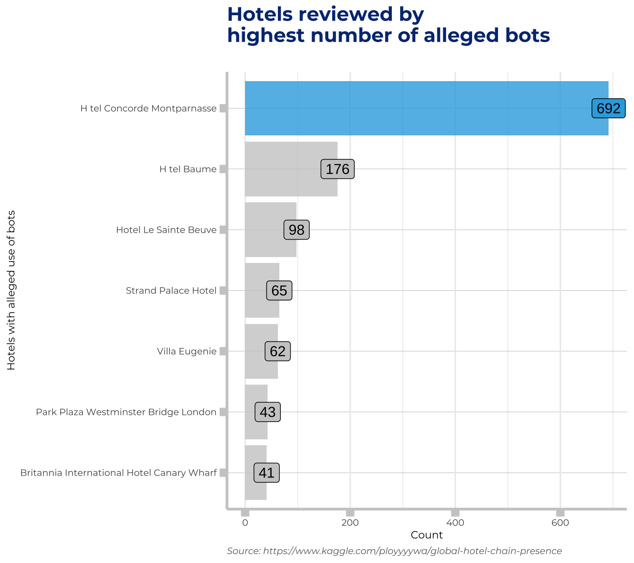
Meaningless reviews vs meaningful reviews
#popularity of bots
bots_by_popularity<-duplicates%>%
  mutate(negative_review_renew=ifelse(negative_review=="No Negative"|negative_review=="Nothing"|negative_review=="nothing"|negative_review=="Everything","Meaningless review","Meaningful review"))%>% #define meaningless review and meaningful review for visualisation
  group_by(negative_review_renew)%>%
  summarise(sum=n())%>%
  arrange(desc(sum))%>%
  mutate(is_others=ifelse(negative_review_renew=="Meaningful review",1,0))%>% #deprecated line, originally used for fill aesthetic colouring, but we cancelled the colouring already
  slice(1:2)

my_text1b <- "No Negative, \nNothing, \nnothing, & \nEverything"
ggplot(bots_by_popularity, aes(x=reorder(negative_review_renew,-sum), y=sum)) +
    geom_bar(stat="identity", alpha=0.8)+
theme_minimal() +
  theme(panel.grid.major.y = element_line(color = "gray60", size = 0.1),
        panel.background = element_rect(fill = "white", colour = "white"),
        axis.line = element_line(size = 1, colour = "grey80"),
        axis.ticks = element_line(size = 3,colour = "grey80"),
        axis.ticks.length = unit(.20, "cm"),
        plot.title = element_text(color = "#043680",size=15,face="bold", family= "Montserrat"),
        plot.subtitle = element_text(color = "#043680", face="plain", ,size= 10,family= "Montserrat"),
        plot.caption = element_text(color = "grey40", face="italic", ,size= 7,family= "Montserrat",hjust=0),
        axis.title.y = element_text(size = 8, angle = 90, family="Montserrat", face = "plain"),
        axis.text.y=element_text(family="Montserrat", size=7),
        axis.title.x = element_text(size = 8, family="Montserrat", face = "plain"),
        axis.text.x=element_text(family="Montserrat", size=7),
        legend.text=element_text(family="Montserrat", size=7),
        legend.title=element_text(family="Montserrat", size=8, face="bold"),
        legend.position = "none")+
    labs(title = "Two-thirds of bots produce meaningless reviews", subtitle= "", x="Type of review", y="Count", caption="(We define repetitive reviews as exactly one of 'No Negative', 'Nothing', 'nothing' and 'Everything')") +
  scale_y_continuous()+
  scale_fill_manual(values = c("grey80"))+
  geom_label(aes(label=sum),family="Montserrat", fontface="bold" )#+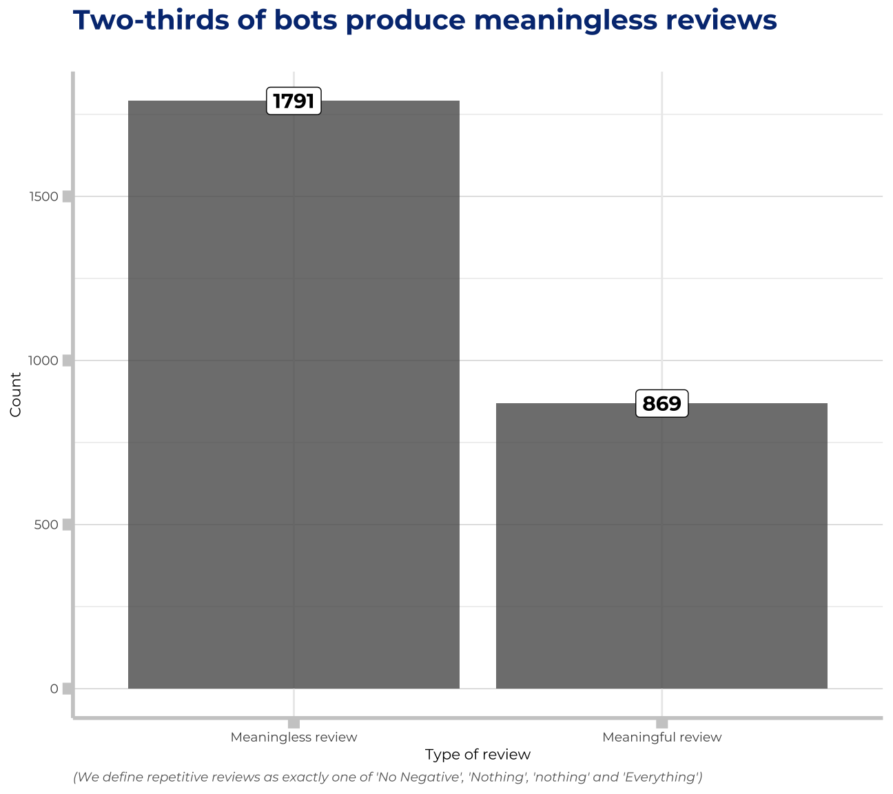
#annotate(geom= "text", x=1.7, y=1500, label=my_text1b, family="Montserrat",size=7, color="#2FABE1",fontface="bold")Thank you!
