Estimation Engine for London House Prices with Stacked Final Model using Tree Models, LASSO, Random Forest & GBM
The purpose of this project is to build an estimation engine to guide investment decisions in London house market. I will first build machine learning algorithms (and tune them) to estimate the house prices given variety of information about each property. Then, using my algorithm, I will choose 200 houses to invest in out of about 2000 houses on the market at the moment.
Objectives
- Using different data mining algorithms for prediction.
- Dealing with large data sets
- Tuning data mining algorithms
- Interpreting data mining algorithms and deducing importance of variables
- Using results of data mining algorithms to make business decisions
Load data
There are two sets of data, i) training data that has the actual prices ii) out of sample data that has the asking prices. I will now load both data sets.
I will make sure to understand what information each column contains. Note that not all information provided might be useful in predicting house prices, but do not make any assumptions before you decide what information you use in your prediction algorithms.
#reading in the data
london_house_prices_2019_training<-read_csv("~/Documents/LBS/Data Science/Session 10/workshop/training_data_assignment_with_prices.csv")
london_house_prices_2019_out_of_sample<-read_csv("~/Documents/LBS/Data Science/Session 10/workshop/test_data_assignment.csv")

#fixing the dates
london_house_prices_2019_out_of_sample<- london_house_prices_2019_out_of_sample %>%
  mutate(date=as.Date(date))

london_house_prices_2019_training<- london_house_prices_2019_training %>%
  mutate(date=as.Date(date))

#changing characters to factors
london_house_prices_2019_out_of_sample <- london_house_prices_2019_out_of_sample %>% mutate_if(is.character, as.factor)

london_house_prices_2019_training <- london_house_prices_2019_training %>% mutate_if(is.character, as.factor)


#making sure out of sample data and training data have the same number of factors
a<-union(levels(london_house_prices_2019_training$postcode_short),levels(london_house_prices_2019_out_of_sample$postcode_short))
london_house_prices_2019_training$postcode_short<- factor(london_house_prices_2019_training$postcode_short,levels=a)
london_house_prices_2019_out_of_sample$postcode_short<-factor(london_house_prices_2019_out_of_sample$postcode_short, levels=a)

b<-union(levels(london_house_prices_2019_training$water_company),levels(london_house_prices_2019_out_of_sample$water_company))
london_house_prices_2019_training$water_company<- factor(london_house_prices_2019_training$water_company,levels=b)
london_house_prices_2019_out_of_sample$water_company<-factor(london_house_prices_2019_out_of_sample$water_company, levels=b)

c<-union(levels(london_house_prices_2019_training$nearest_station),levels(london_house_prices_2019_out_of_sample$nearest_station))
london_house_prices_2019_training$nearest_station<- factor(london_house_prices_2019_training$nearest_station,levels=c)
london_house_prices_2019_out_of_sample$nearest_station<-factor(london_house_prices_2019_out_of_sample$nearest_station, levels=c)

d<-union(levels(london_house_prices_2019_training$district),levels(london_house_prices_2019_out_of_sample$district))
london_house_prices_2019_training$district<- factor(london_house_prices_2019_training$district,levels=d)
london_house_prices_2019_out_of_sample$district<-factor(london_house_prices_2019_out_of_sample$district, levels=d)


#take a quick look at what's in the data
str(london_house_prices_2019_training)
## tibble [13,998 × 37] (S3: spec_tbl_df/tbl_df/tbl/data.frame)
## $ ID : num [1:13998] 2 3 4 5 7 8 9 10 11 12 ...
## $ date : Date[1:13998], format: "2019-11-01" "2019-08-08" ...
## $ postcode : Factor w/ 12635 levels "BR1 1AB","BR1 1LR",..: 10897 11027 11264 2031 11241 11066 421 9594 9444 873 ...
## $ property_type : Factor w/ 4 levels "D","F","S","T": 2 2 3 2 3 2 1 4 4 2 ...
## $ whether_old_or_new : Factor w/ 2 levels "N","Y": 1 1 1 1 1 1 1 1 1 1 ...
## $ freehold_or_leasehold : Factor w/ 2 levels "F","L": 2 2 1 2 1 2 1 1 1 2 ...
## $ address1 : Factor w/ 2825 levels "1","1 - 2","1 - 3",..: 2503 792 253 789 569 234 264 418 5 274 ...
## $ address2 : Factor w/ 434 levels "1","10","101",..: 372 NA NA NA NA NA NA NA NA NA ...
## $ address3 : Factor w/ 8543 levels "ABBERTON WALK",..: 6990 6821 3715 2492 4168 2879 3620 5251 6045 6892 ...
## $ town : Factor w/ 133 levels "ABBEY WOOD","ACTON",..: NA NA NA 78 NA NA NA NA NA NA ...
## $ local_aut : Factor w/ 69 levels "ASHFORD","BARKING",..: 36 46 24 36 24 46 65 36 36 17 ...
## $ county : Factor w/ 33 levels "BARKING AND DAGENHAM",..: 22 27 18 25 18 27 5 27 32 8 ...
## $ postcode_short : Factor w/ 248 levels "BR1","BR2","BR3",..: 190 194 198 28 198 194 4 169 167 8 ...
## $ current_energy_rating : Factor w/ 6 levels "B","C","D","E",..: 4 3 3 4 3 2 4 3 4 2 ...
## $ total_floor_area : num [1:13998] 30 50 100 39 88 101 136 148 186 65 ...
## $ number_habitable_rooms : num [1:13998] 2 2 5 2 4 4 6 6 6 3 ...
## $ co2_emissions_current : num [1:13998] 2.3 3 3.7 2.8 3.9 3.1 8.1 5.6 10 1.5 ...
## $ co2_emissions_potential : num [1:13998] 1.7 1.7 1.5 1.1 1.4 1.4 4.1 2 6.1 1.5 ...
## $ energy_consumption_current : num [1:13998] 463 313 212 374 251 175 339 216 308 128 ...
## $ energy_consumption_potential: num [1:13998] 344 175 82 144 90 77 168 75 186 128 ...
## $ windows_energy_eff : Factor w/ 5 levels "Average","Good",..: 1 1 1 5 1 1 1 1 5 1 ...
## $ tenure : Factor w/ 3 levels "owner-occupied",..: 1 2 1 2 1 1 1 2 1 1 ...
## $ latitude : num [1:13998] 51.5 51.5 51.5 51.6 51.5 ...
## $ longitude : num [1:13998] -0.1229 -0.2828 -0.4315 0.0423 -0.4293 ...
## $ population : num [1:13998] 34 75 83 211 73 51 25 91 60 97 ...
## $ altitude : num [1:13998] 8 9 25 11 21 11 95 7 7 106 ...
## $ london_zone : num [1:13998] 1 3 5 3 6 6 3 2 2 3 ...
## $ nearest_station : Factor w/ 594 levels "abbey road","abbey wood",..: 478 358 235 319 180 502 566 30 32 566 ...
## $ water_company : Factor w/ 5 levels "Affinity Water",..: 5 5 1 5 1 5 5 5 5 5 ...
## $ average_income : num [1:13998] 57200 61900 50600 45400 49000 56200 57200 65600 50400 52300 ...
## $ district : Factor w/ 33 levels "Barking and Dagenham",..: 22 27 18 26 18 27 5 27 32 8 ...
## $ price : num [1:13998] 360000 408500 499950 259999 395000 ...
## $ type_of_closest_station : Factor w/ 3 levels "light_rail","rail",..: 3 2 3 1 3 2 1 3 1 1 ...
## $ num_tube_lines : num [1:13998] 1 0 1 0 1 0 0 2 0 0 ...
## $ num_rail_lines : num [1:13998] 0 1 1 0 1 1 0 0 1 0 ...
## $ num_light_rail_lines : num [1:13998] 0 0 0 1 0 0 1 0 1 1 ...
## $ distance_to_station : num [1:13998] 0.528 0.77 0.853 0.29 1.073 ...
## - attr(*, "spec")=
## .. cols(
## .. ID = col_double(),
## .. date = col_date(format = ""),
## .. postcode = col_character(),
## .. property_type = col_character(),
## .. whether_old_or_new = col_character(),
## .. freehold_or_leasehold = col_character(),
## .. address1 = col_character(),
## .. address2 = col_character(),
## .. address3 = col_character(),
## .. town = col_character(),
## .. local_aut = col_character(),
## .. county = col_character(),
## .. postcode_short = col_character(),
## .. current_energy_rating = col_character(),
## .. total_floor_area = col_double(),
## .. number_habitable_rooms = col_double(),
## .. co2_emissions_current = col_double(),
## .. co2_emissions_potential = col_double(),
## .. energy_consumption_current = col_double(),
## .. energy_consumption_potential = col_double(),
## .. windows_energy_eff = col_character(),
## .. tenure = col_character(),
## .. latitude = col_double(),
## .. longitude = col_double(),
## .. population = col_double(),
## .. altitude = col_double(),
## .. london_zone = col_double(),
## .. nearest_station = col_character(),
## .. water_company = col_character(),
## .. average_income = col_double(),
## .. district = col_character(),
## .. price = col_double(),
## .. type_of_closest_station = col_character(),
## .. num_tube_lines = col_double(),
## .. num_rail_lines = col_double(),
## .. num_light_rail_lines = col_double(),
## .. distance_to_station = col_double()
## .. )str(london_house_prices_2019_out_of_sample)## tibble [1,999 × 37] (S3: spec_tbl_df/tbl_df/tbl/data.frame)
## $ ID : num [1:1999] 14434 12562 8866 10721 1057 ...
## $ date : Date[1:1999], format: NA NA ...
## $ postcode : logi [1:1999] NA NA NA NA NA NA ...
## $ property_type : Factor w/ 4 levels "D","F","S","T": 1 2 2 3 4 3 2 3 2 4 ...
## $ whether_old_or_new : Factor w/ 2 levels "N","Y": 1 1 1 1 1 1 1 1 1 1 ...
## $ freehold_or_leasehold : Factor w/ 2 levels "F","L": 1 2 2 1 1 1 2 1 2 1 ...
## $ address1 : logi [1:1999] NA NA NA NA NA NA ...
## $ address2 : logi [1:1999] NA NA NA NA NA NA ...
## $ address3 : logi [1:1999] NA NA NA NA NA NA ...
## $ town : Factor w/ 54 levels "ACTON","ADDISCOMBE",..: NA NA NA NA NA NA NA NA NA NA ...
## $ local_aut : logi [1:1999] NA NA NA NA NA NA ...
## $ county : logi [1:1999] NA NA NA NA NA NA ...
## $ postcode_short : Factor w/ 248 levels "BR1","BR2","BR3",..: 91 58 37 60 232 159 168 124 187 135 ...
## $ current_energy_rating : Factor w/ 6 levels "B","C","D","E",..: 3 2 3 3 4 4 4 3 4 3 ...
## $ total_floor_area : num [1:1999] 150 59 58 74 97.3 ...
## $ number_habitable_rooms : num [1:1999] 6 2 2 5 5 5 5 4 2 5 ...
## $ co2_emissions_current : num [1:1999] 7.3 1.5 2.8 3.5 6.5 4.9 5.1 2.9 4.2 4.3 ...
## $ co2_emissions_potential : num [1:1999] 2.4 1.4 1.2 1.2 5.7 1.6 3 0.8 3.2 2.5 ...
## $ energy_consumption_current : num [1:1999] 274 142 253 256 303 309 240 224 458 253 ...
## $ energy_consumption_potential: num [1:1999] 89 136 110 80 266 101 140 58 357 143 ...
## $ windows_energy_eff : Factor w/ 5 levels "Average","Good",..: 1 1 1 1 1 1 3 1 3 1 ...
## $ tenure : Factor w/ 3 levels "owner-occupied",..: 1 1 1 1 1 1 1 1 1 1 ...
## $ latitude : num [1:1999] 51.6 51.6 51.5 51.6 51.5 ...
## $ longitude : num [1:1999] -0.129 -0.2966 -0.0328 -0.3744 -0.2576 ...
## $ population : num [1:1999] 87 79 23 73 100 24 22 49 65 98 ...
## $ altitude : num [1:1999] 63 38 17 39 8 46 26 16 14 18 ...
## $ london_zone : num [1:1999] 4 4 2 5 2 4 3 6 1 3 ...
## $ nearest_station : Factor w/ 594 levels "abbey road","abbey wood",..: 19 546 214 362 516 168 24 519 148 251 ...
## $ water_company : Factor w/ 5 levels "Affinity Water",..: 5 1 5 1 5 5 5 2 5 5 ...
## $ average_income : num [1:1999] 61300 48900 46200 52200 60700 59600 64000 48100 56600 53500 ...
## $ district : Factor w/ 33 levels "Barking and Dagenham",..: 10 4 30 15 18 11 32 16 20 23 ...
## $ type_of_closest_station : Factor w/ 3 levels "light_rail","rail",..: 3 3 1 2 3 2 3 3 3 2 ...
## $ num_tube_lines : num [1:1999] 1 2 0 0 2 0 1 1 2 0 ...
## $ num_rail_lines : num [1:1999] 0 1 0 1 0 1 1 0 0 1 ...
## $ num_light_rail_lines : num [1:1999] 0 1 1 0 0 0 0 1 0 0 ...
## $ distance_to_station : num [1:1999] 0.839 0.104 0.914 0.766 0.449 ...
## $ asking_price : num [1:1999] 750000 229000 152000 379000 930000 350000 688000 386000 534000 459000 ...
## - attr(*, "spec")=
## .. cols(
## .. ID = col_double(),
## .. date = col_logical(),
## .. postcode = col_logical(),
## .. property_type = col_character(),
## .. whether_old_or_new = col_character(),
## .. freehold_or_leasehold = col_character(),
## .. address1 = col_logical(),
## .. address2 = col_logical(),
## .. address3 = col_logical(),
## .. town = col_character(),
## .. local_aut = col_logical(),
## .. county = col_logical(),
## .. postcode_short = col_character(),
## .. current_energy_rating = col_character(),
## .. total_floor_area = col_double(),
## .. number_habitable_rooms = col_double(),
## .. co2_emissions_current = col_double(),
## .. co2_emissions_potential = col_double(),
## .. energy_consumption_current = col_double(),
## .. energy_consumption_potential = col_double(),
## .. windows_energy_eff = col_character(),
## .. tenure = col_character(),
## .. latitude = col_double(),
## .. longitude = col_double(),
## .. population = col_double(),
## .. altitude = col_double(),
## .. london_zone = col_double(),
## .. nearest_station = col_character(),
## .. water_company = col_character(),
## .. average_income = col_double(),
## .. district = col_character(),
## .. type_of_closest_station = col_character(),
## .. num_tube_lines = col_double(),
## .. num_rail_lines = col_double(),
## .. num_light_rail_lines = col_double(),
## .. distance_to_station = col_double(),
## .. asking_price = col_double()
## .. )#describe(london_house_prices_2019_training)In my predictions, I will not use columns between date:country. For the rest of variables, I will investigate their performance and correlation to price in further steps.
#let's do the initial split
set.seed(1)
train_test_split <- initial_split(london_house_prices_2019_training, prop = 0.75) #training set contains 75% of the data
set.seed(1)
# Create the training dataset
train_data <- training(train_test_split)
# Create the testing dataset
test_data <- testing(train_test_split)
Visualize data
In this section I will visualise my data. The most useful plots will tackle factor variables from our dataset, as the numeric ones we can examine later on in the correlation matrix.
#checking the data once again
#summary(train_data)
#glimpse(train_data)

# avg price in districts
train_data_vis1 <- train_data %>%
  group_by(district) %>%
  summarise(avg = mean(price))


vis1 <- train_data_vis1 %>%
  ggplot (aes(y=avg, x=reorder(district,avg))) +
            geom_col() +
  coord_flip() +
  theme_bw() +
  theme(panel.grid.major.y = element_line(color = "gray60", size = 0.1),
        panel.background = element_rect(fill = "white", colour = "white"),
        axis.line = element_line(size = 1, colour = "grey80"),
        axis.ticks = element_line(size = 3,colour = "grey80"),
        plot.title = element_text(color = "grey80",size=15,face="bold", family= "Montserrat"),
        axis.title.y = element_text(size = 8, angle = 90, family="Montserrat", face = "bold"),
        axis.text.y=element_text(family="Montserrat", size=7),
        axis.title.x = element_text(size = 8, family="Montserrat", face = "bold"),
        axis.text.x=element_text(family="Montserrat", size=7))+
    labs(y="Price", x="London district")

vis1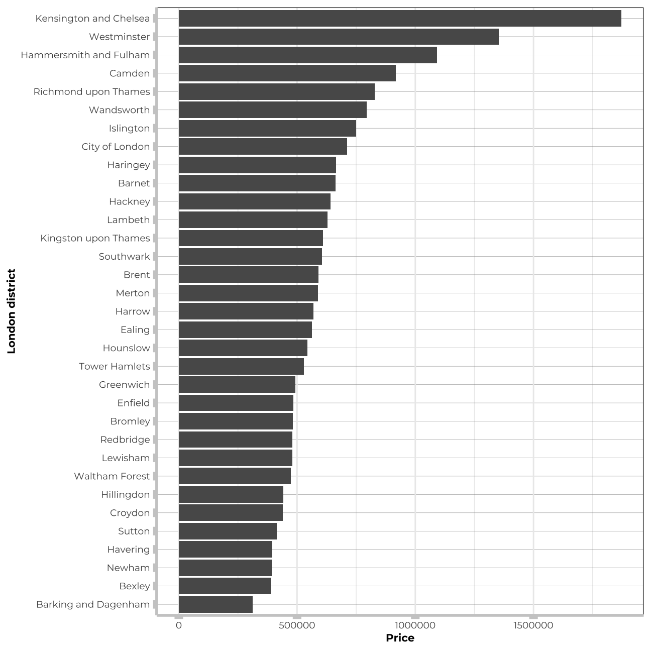
#avg price vs nearest station

train_data_vis2 <- train_data %>%
  group_by(nearest_station) %>%
  summarise(avg = mean(price))

train_data_vis2<-train_data_vis2 %>%
    arrange(desc(avg)) %>%
    filter(avg>2000000)


vis2 <- train_data_vis2 %>%
  ggplot (aes(y=avg, x=reorder(nearest_station,avg))) +
            geom_col() +
  coord_flip() +
  theme_bw() +
  theme(panel.grid.major.y = element_line(color = "gray60", size = 0.1),
        panel.background = element_rect(fill = "white", colour = "white"),
        axis.line = element_line(size = 1, colour = "grey80"),
        axis.ticks = element_line(size = 3,colour = "grey80"),
        plot.title = element_text(color = "grey80",size=15,face="bold", family= "Montserrat"),
        axis.title.y = element_text(size = 8, angle = 90, family="Montserrat", face = "bold"),
        axis.text.y=element_text(family="Montserrat", size=7),
        axis.title.x = element_text(size = 8, family="Montserrat", face = "bold"),
        axis.text.x=element_text(family="Montserrat", size=7))+
    labs(y="Price", x="Nearest station")


vis2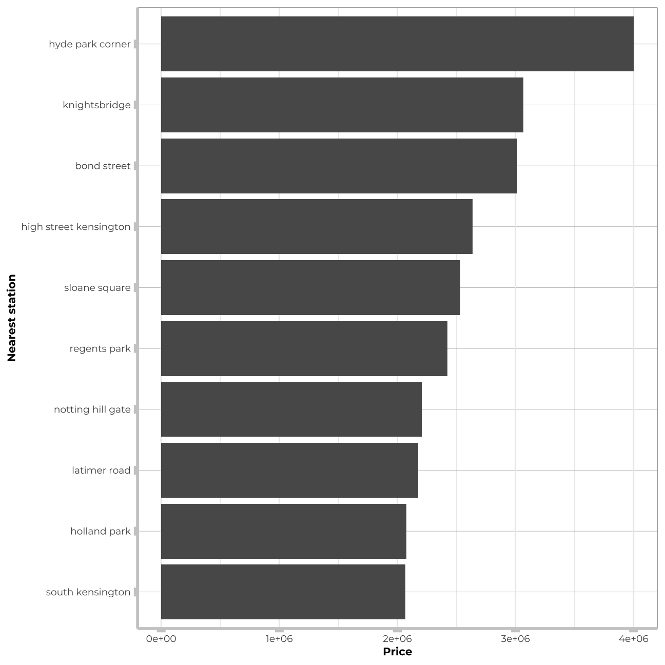
#Graph showing price in ths in particular property types  in regards to different london zones and station types

train_data_vis3 <- train_data %>%
  group_by(type_of_closest_station, property_type, london_zone) %>%
  summarise(avg = mean(price))

train_data_vis3$property_type<- train_data_vis3$property_type %>% factor(levels=c("D","S", "T", "F"))

vis3 <- train_data_vis3 %>%
  ggplot(aes(y=avg, x=property_type,fill=property_type))+
  geom_col() +
  facet_grid(type_of_closest_station~london_zone)+
  theme_bw() +
  theme(panel.grid.major.y = element_line(color = "gray60", size = 0.1),
        strip.text= element_text(family="Montserrat", face = "plain"),
        panel.background = element_rect(fill = "white", colour = "white"),
        axis.line = element_line(size = 1, colour = "grey80"),
        axis.ticks = element_line(size = 3,colour = "grey80"),
        axis.ticks.length = unit(.20, "cm"),
        plot.title = element_text(color = "grey40",size=10,face="bold", family= "Montserrat"),
        plot.caption = element_text(color = "grey40", face="italic",size= 7,family= "Montserrat",hjust=0),
        axis.title.y = element_text(size = 8, angle = 90, family="Montserrat", face = "bold"),
        axis.text.y=element_text(family="Montserrat", size=7),
        axis.title.x = element_text(size = 8, family="Montserrat", face = "bold"),
        axis.text.x=element_text(family="Montserrat", size=7),
        legend.text=element_text(family="Montserrat", size=7),
        legend.title=element_text(family="Montserrat", size=8, face="bold")
                                  )+
    labs(title="Average price in regards to proerty types located in \nparticular london zones near specific types of stations",y="Price", x="Property type") +
  scale_fill_discrete(name = "Property type", labels = c("Detached", "Semi-detached", "Terraced", "Flat/Masionette"))

vis3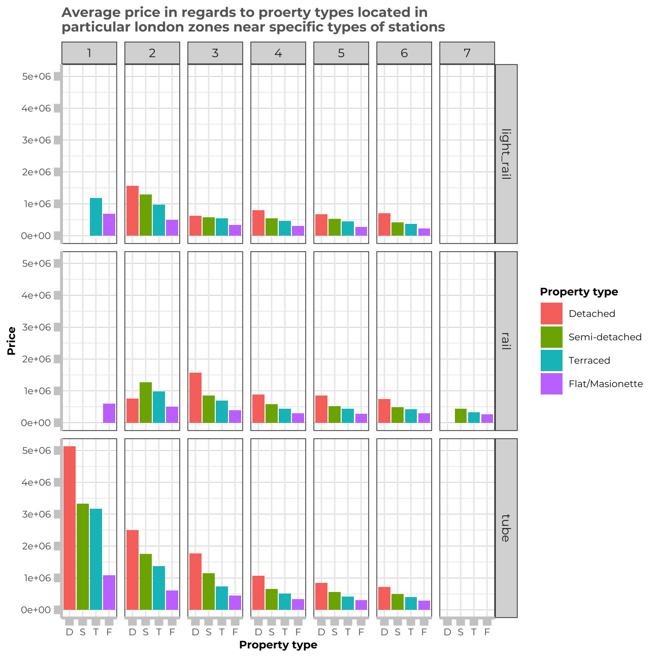
# price vs distance to the station & propety_type
train_data_vis4 <- train_data %>%
  group_by(property_type, distance_to_station) %>%
  summarise(avg = mean(price))

vis4 <- train_data_vis4 %>%
  ggplot(aes(y=avg, x=distance_to_station))+
  geom_point()+
  facet_wrap(~property_type)


vis4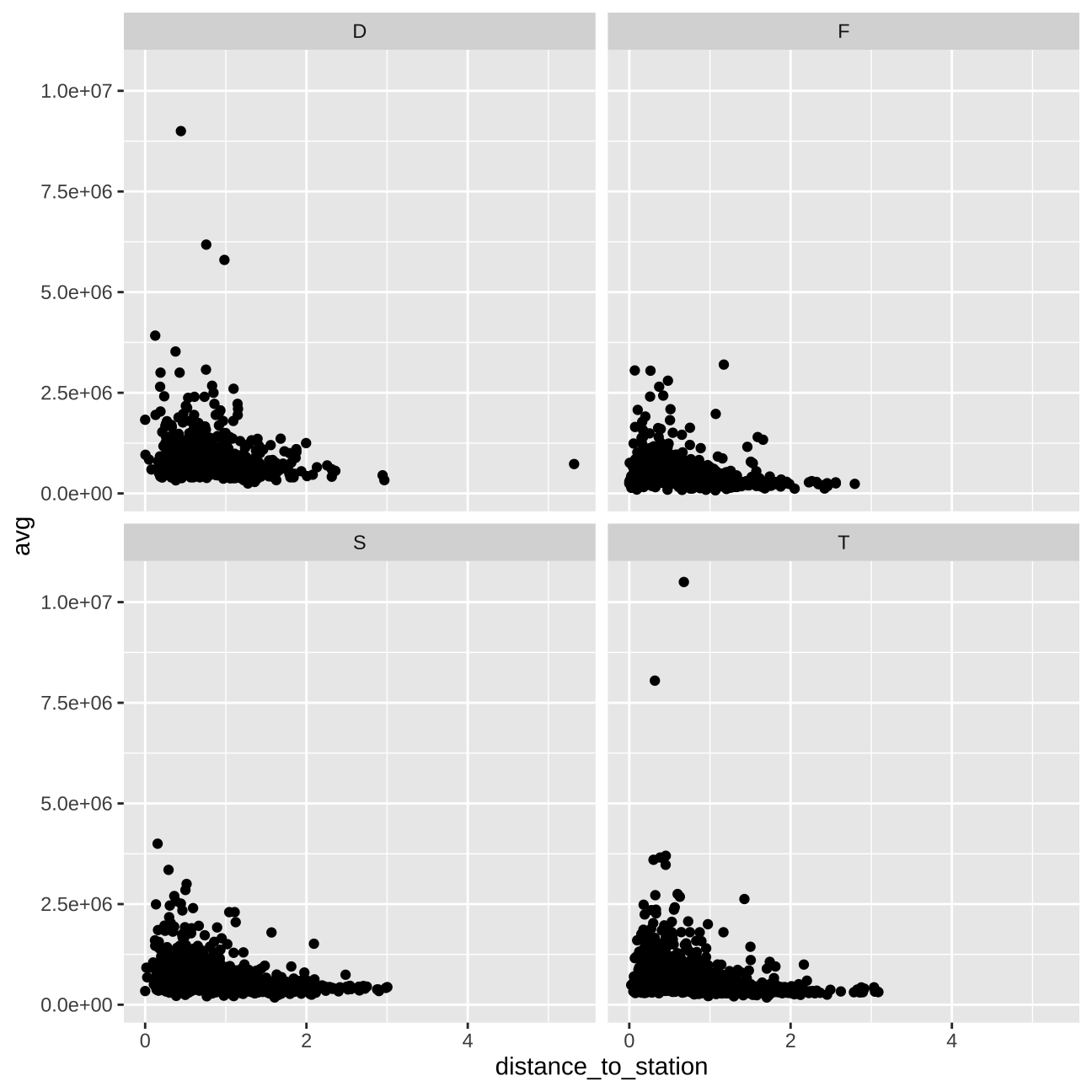
# energy_ratings vs price
train_data_vis5 <- train_data %>%
  group_by(current_energy_rating) %>%
  summarise(avg = mean(price))

vis5 <- train_data_vis5 %>%
  ggplot(aes(y=avg, x=current_energy_rating))+
  geom_col()

vis5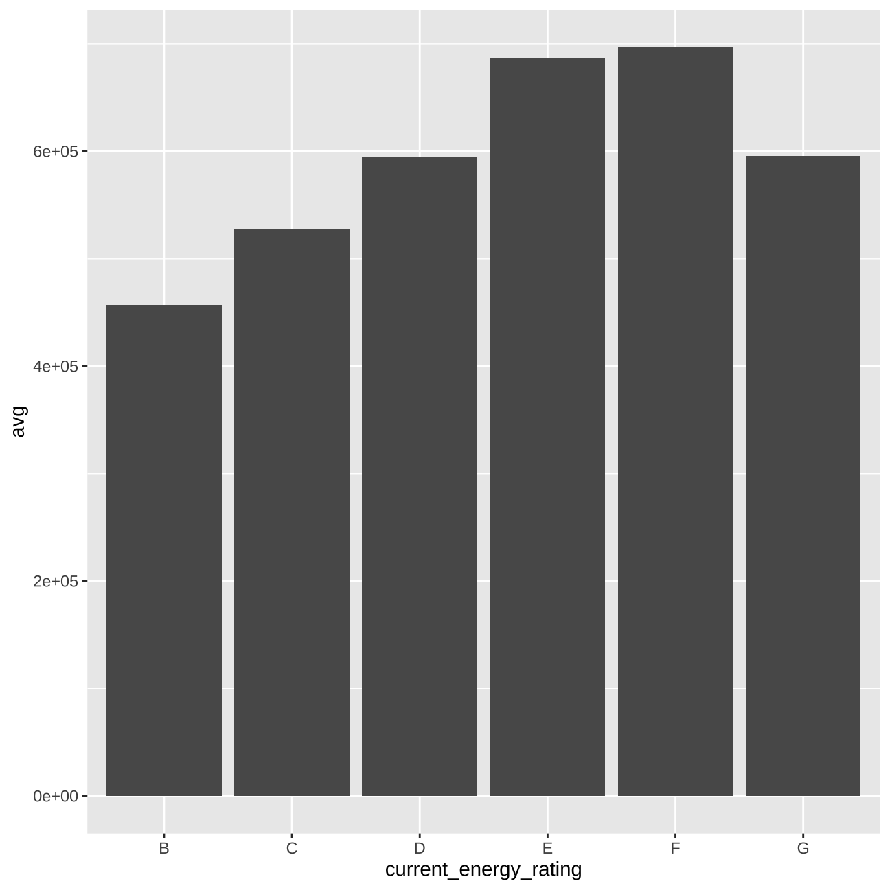
#correlations
vis6<- train_data %>%
  select(distance_to_station, london_zone, price,) %>% #order variables they will appear in ggpairs()
  ggpairs(aes(alpha = 0.3))+
  theme_bw()

vis6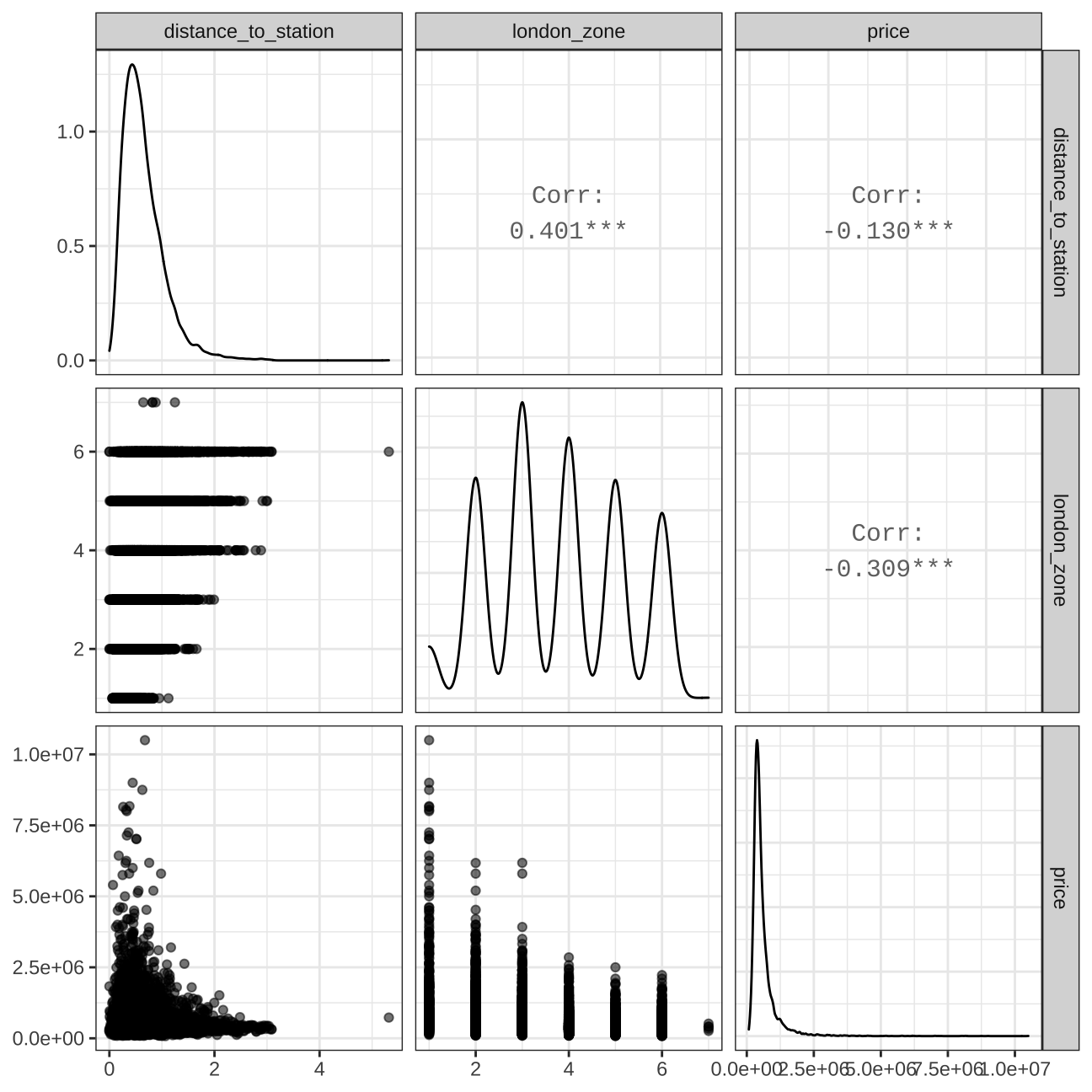
#price vs water_provider
train_data_vis7 <- train_data %>%
  group_by(water_company) %>%
  summarise(avg = mean(price))


vis7 <- train_data_vis7 %>%
  ggplot (aes(y=avg, x=reorder(water_company,avg))) +
            geom_col() +
  coord_flip()

vis7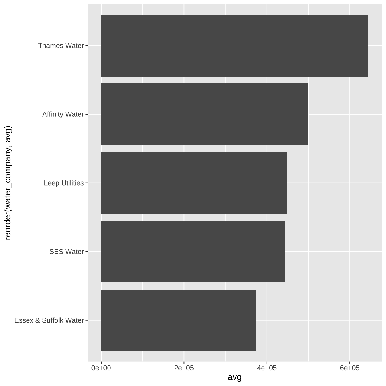
#price vs freehold_or_leasehold
train_data_vis8 <- train_data %>%
  group_by(freehold_or_leasehold) %>%
  summarise(avg = mean(price))


vis8 <- train_data_vis8 %>%
  ggplot (aes(y=avg, x=reorder(freehold_or_leasehold,avg))) +
            geom_col() +
  coord_flip()

vis8
#price vs windows_energy_eff
train_data_vis9 <- train_data %>%
  group_by(windows_energy_eff) %>%
  summarise(avg = mean(price))


vis9 <- train_data_vis9 %>%
  ggplot (aes(y=avg, x=reorder(windows_energy_eff,avg))) +
            geom_col() +
  coord_flip()

vis9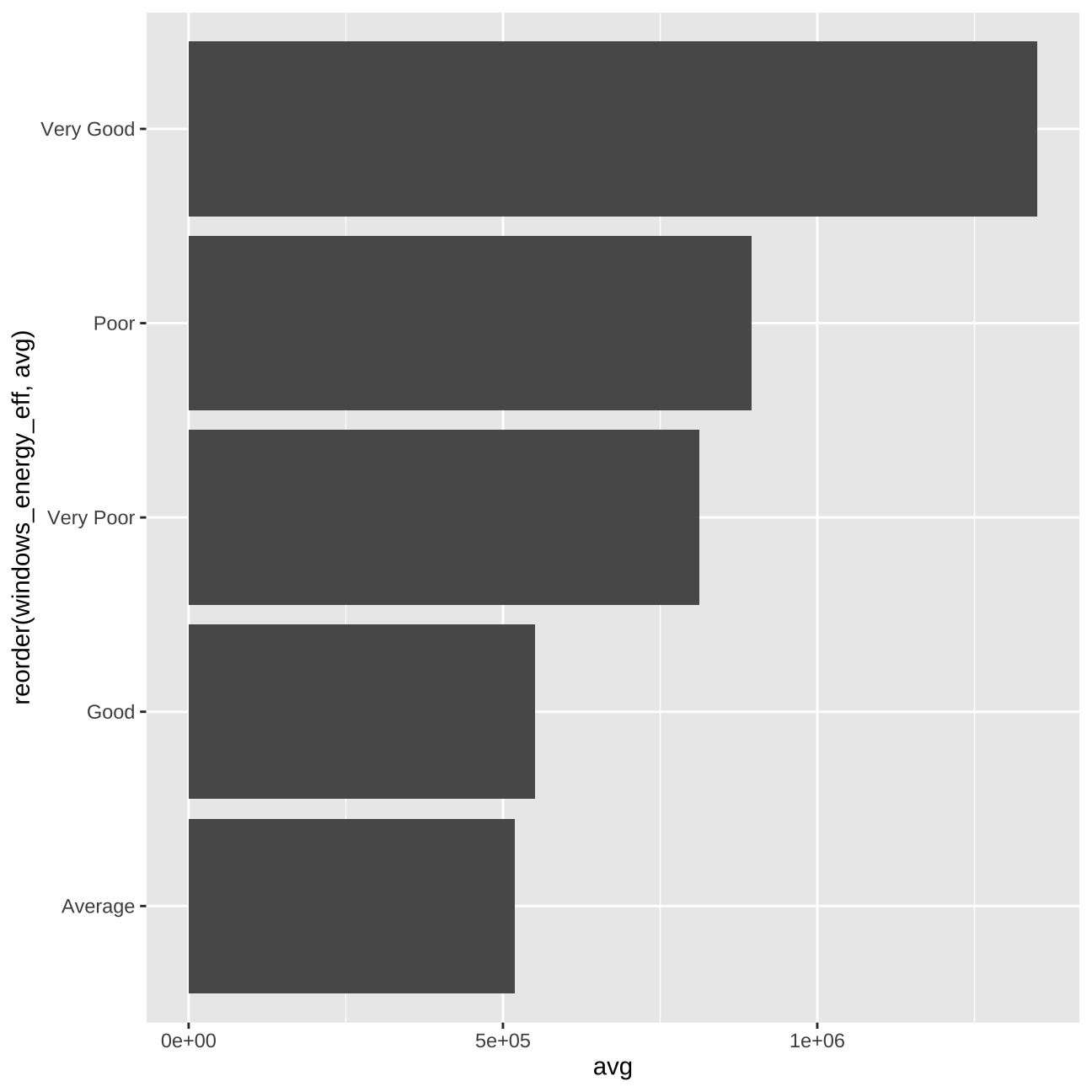
#price vs tenure
train_data_vis10 <- train_data %>%
  group_by(tenure ) %>%
  summarise(avg = mean(price))


vis10 <- train_data_vis10 %>%
  ggplot (aes(y=avg, x=reorder(tenure ,avg))) +
            geom_col() +
  coord_flip()

vis10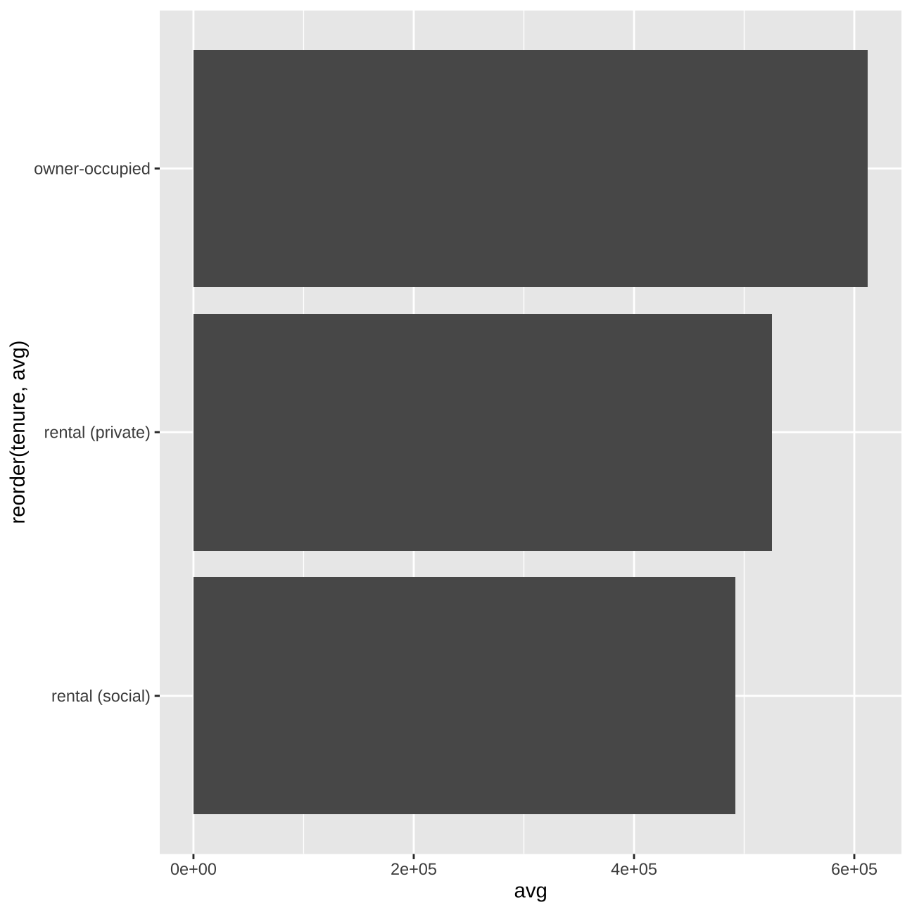
#postcode_short
train_data_vis11 <- train_data %>%
  group_by(postcode_short) %>%
  summarise(avg = mean(price)) %>%
  arrange(desc(avg)) %>%
  filter(avg>2000000)


vis11<- train_data_vis11 %>%
  ggplot (aes(y=avg, x=reorder(postcode_short,avg))) +
            geom_col() +
  coord_flip()+
  theme_bw() +
  theme(panel.grid.major.y = element_line(color = "gray60", size = 0.1),
        panel.background = element_rect(fill = "white", colour = "white"),
        axis.line = element_line(size = 1, colour = "grey80"),
        axis.ticks = element_line(size = 3,colour = "grey80"),
        plot.title = element_text(color = "grey80",size=15,face="bold", family= "Montserrat"),
        axis.title.y = element_text(size = 8, angle = 90, family="Montserrat", face = "bold"),
        axis.text.y=element_text(family="Montserrat", size=7),
        axis.title.x = element_text(size = 8, family="Montserrat", face = "bold"),
        axis.text.x=element_text(family="Montserrat", size=7))+
    labs(y="Price", x="Postcode short version")

vis11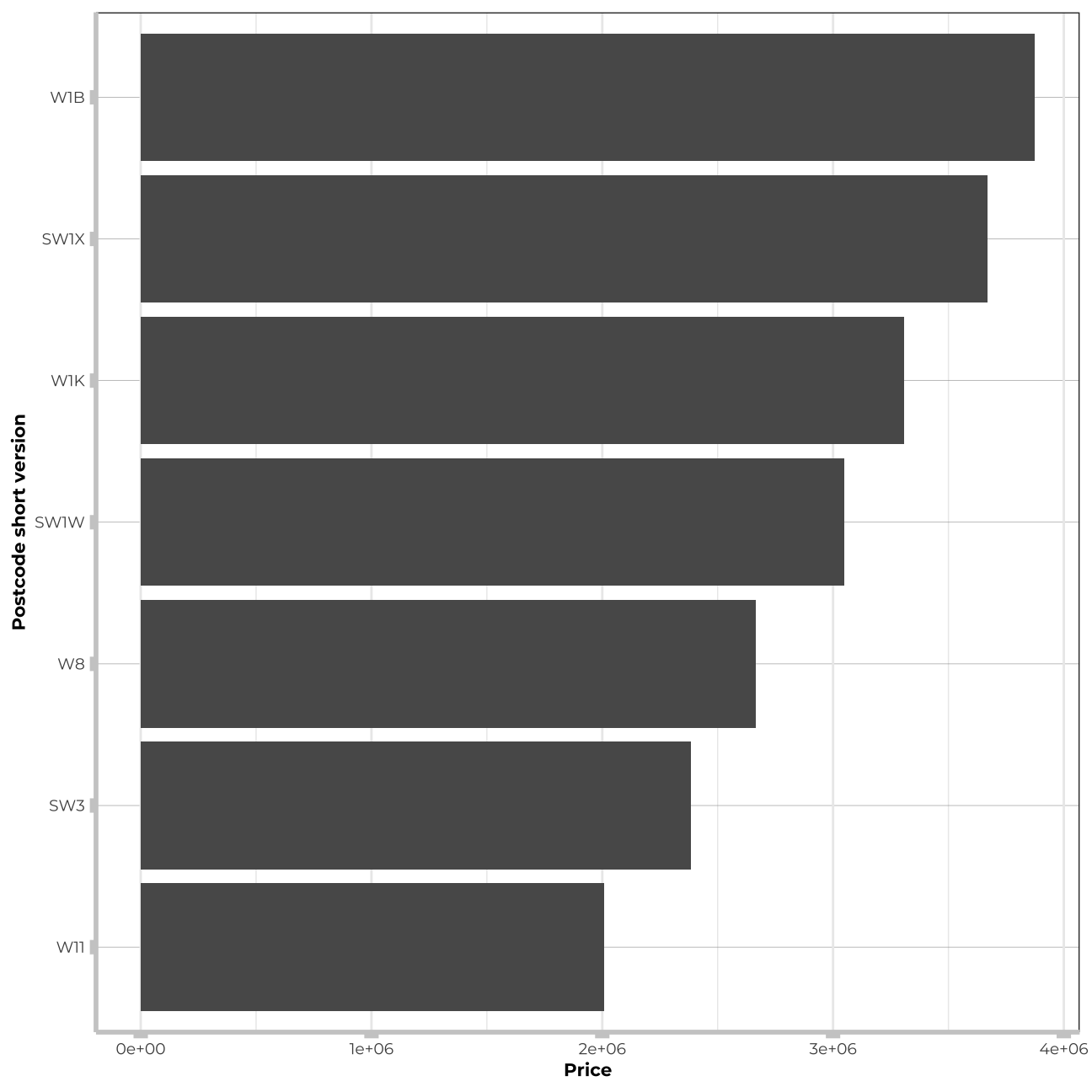
train_data_vis12 <- train_data %>%
  group_by(total_floor_area,london_zone) %>%
  summarise(avg = mean(price)) %>%
  arrange(desc(avg))

vis12<-train_data_vis12%>%
  ggplot(aes(x=total_floor_area, y=avg))+
  geom_smooth() +
  facet_wrap(~london_zone)+
  theme_bw() +
  theme(panel.grid.major.y = element_line(color = "gray60", size = 0.1),
        strip.text= element_text(family="Montserrat", face = "plain"),
        panel.background = element_rect(fill = "white", colour = "white"),
        axis.line = element_line(size = 1, colour = "grey80"),
        axis.ticks = element_line(size = 3,colour = "grey80"),
        axis.ticks.length = unit(.20, "cm"),
        plot.title = element_text(color = "grey40",size=10,face="bold", family= "Montserrat"),
        plot.caption = element_text(color = "grey40", face="italic",size= 7,family= "Montserrat",hjust=0),
        axis.title.y = element_text(size = 8, angle = 90, family="Montserrat", face = "bold"),
        axis.text.y=element_text(family="Montserrat", size=7),
        axis.title.x = element_text(size = 8, family="Montserrat", face = "bold"),
        axis.text.x=element_text(family="Montserrat", size=7),
        legend.text=element_text(family="Montserrat", size=7),
        legend.title=element_text(family="Montserrat", size=8, face="bold"))+
    labs(title= "Changes in average Price in regards to total floor area & london_zone", y="Price", x="Total floor area in particular London zone")


vis12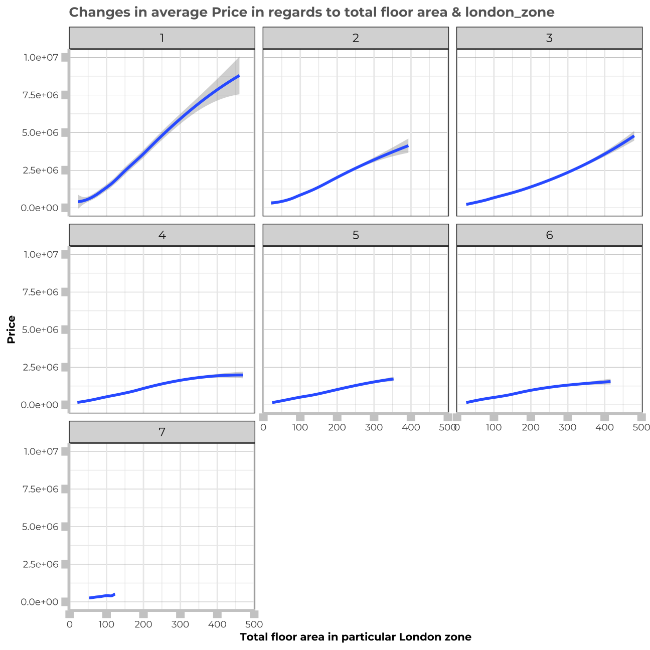
Learnings from visualisations
It seems that the price of houses located in the most distinguished districts in London is significantly affected and much higher than in other districts - the same trend tackles the most popular and best located tube stations and postcodes_short.. Therefore, I will create three new varaibles in my data:-
is_district: that will have value “TRUE” for the most expensive districts and “FALSE” for the rest -
is_station: that will take the value “TRUE” for the station where house price was above 2,000,000. -
is_postcode: that will take the value “TRUE” for the postcode_short where house price exceeded 2,000,000.
Additionally, we can learn from the visualisations, that property_type and distance to the station combined also have a significant influence on the price. Also, london_zone and distance_to_station seem to be interconnected.
When in comes to such variables as “current_energy_rating”, “freehold_or_leasehold”, or“tenure”, we will need to deduct from the further models if any values are really significant for estimating the price or not.
From the graphs, we can deduct that for “water_company” and “windows_energy_eff” only one value of each variable seems to affect the price significantly. We will further exemine it in the next steps.
Feature engineering
I will now add new variables to my dayaset basing on what I found in the section above.
#Adding variable "is station" for stations beloning to the one near which the price of a property sis significantly bigger (assumption: over 2,000,000)
train_data<- train_data %>%
mutate(is_station = ifelse(nearest_station == "hyde park corner" |
                             nearest_station == "   knightsbridge" |
                             nearest_station == "south kensington" |
                             nearest_station == "   holland park" |
                             nearest_station == "bond street"|
                             nearest_station == "regents park"|
                             nearest_station == "high street kensington"|
                             nearest_station == "gloucester road"|
                             nearest_station == "sloane square", TRUE, FALSE ))

test_data<- test_data %>%
mutate(is_station = ifelse(nearest_station == "hyde park corner" |
                             nearest_station == "   knightsbridge" |
                             nearest_station == "south kensington" |
                             nearest_station == "   holland park" |
                             nearest_station == "bond street"|
                             nearest_station == "regents park"|
                             nearest_station == "high street kensington"|
                             nearest_station == "gloucester road"|
                             nearest_station == "sloane square", TRUE, FALSE ))

london_house_prices_2019_out_of_sample<- london_house_prices_2019_out_of_sample %>%
mutate(is_station = ifelse(nearest_station == "hyde park corner" |
                             nearest_station == "   knightsbridge" |
                             nearest_station == "south kensington" |
                             nearest_station == "   holland park" |
                             nearest_station == "bond street"|
                             nearest_station == "regents park"|
                             nearest_station == "high street kensington"|
                             nearest_station == "gloucester road"|
                             nearest_station == "sloane square", TRUE, FALSE ))


#Adding a variable is_district with 5 most expensive districts in London
train_data<- train_data %>%
mutate(is_district = ifelse(district == "Kensington and Chelsea" |
                              district == "Westminster" |
                              district == "Hammersmith and Fulham" |
                              district == "Camden" |
                              district == "Richmond upon Thames", TRUE, FALSE ))

test_data<- test_data %>%
mutate(is_district = ifelse(district == "Kensington and Chelsea" |
                              district == "Westminster" |
                              district == "Hammersmith and Fulham" |
                              district == "Camden" |
                              district == "Richmond upon Thames", TRUE, FALSE ))


london_house_prices_2019_out_of_sample<- london_house_prices_2019_out_of_sample %>%
mutate(is_district = ifelse(district == "Kensington and Chelsea" |
                              district == "Westminster" |
                              district == "Hammersmith and Fulham" |
                              district == "Camden" |
                              district == "Richmond upon Thames", TRUE, FALSE ))

#Adding a variable is_postcode with 6 most expensive postcodes in London
train_data<- train_data %>%
mutate(is_postcode = ifelse(postcode_short == "W1B" |
                             postcode_short == "    SW1X" |
                             postcode_short == "W1K" |
                             postcode_short == "SW1W" |
                             postcode_short == "W8"|
                             postcode_short == "S3"|
                              postcode_short == "W11", TRUE, FALSE ))

test_data<- test_data %>%
mutate(is_postcode = ifelse(postcode_short == "W1B" |
                             postcode_short == "    SW1X" |
                             postcode_short == "W1K" |
                             postcode_short == "SW1W" |
                             postcode_short == "W8"|
                             postcode_short == "S3"|
                              postcode_short == "W11", TRUE, FALSE ))

london_house_prices_2019_out_of_sample<- london_house_prices_2019_out_of_sample %>%
mutate(is_postcode = ifelse(postcode_short == "W1B" |
                             postcode_short == "    SW1X" |
                             postcode_short == "W1K" |
                             postcode_short == "SW1W" |
                             postcode_short == "W8"|
                             postcode_short == "S3"|
                              postcode_short == "W11", TRUE, FALSE ))
Distribution of dependent variable
I will now check the distirbution of the “price” variable to check if it follows the Normal distribution.
#distribution of price
train_data %>%
  ggplot(aes(x=price))+
  geom_histogram()+
  theme_bw() +
  theme(panel.grid.major.y = element_line(color = "gray60", size = 0.1),
        panel.background = element_rect(fill = "white", colour = "white"),
        axis.line = element_line(size = 1, colour = "grey80"),
        axis.ticks = element_line(size = 3,colour = "grey80"),
        plot.title = element_text(color = "grey80",size=15,face="bold", family= "Montserrat"),
        axis.title.y = element_text(size = 8, angle = 90, family="Montserrat", face = "bold"),
        axis.text.y=element_text(family="Montserrat", size=7),
        axis.title.x = element_text(size = 8, family="Montserrat", face = "bold"),
        axis.text.x=element_text(family="Montserrat", size=7))+
labs(x="Price", y="Count") 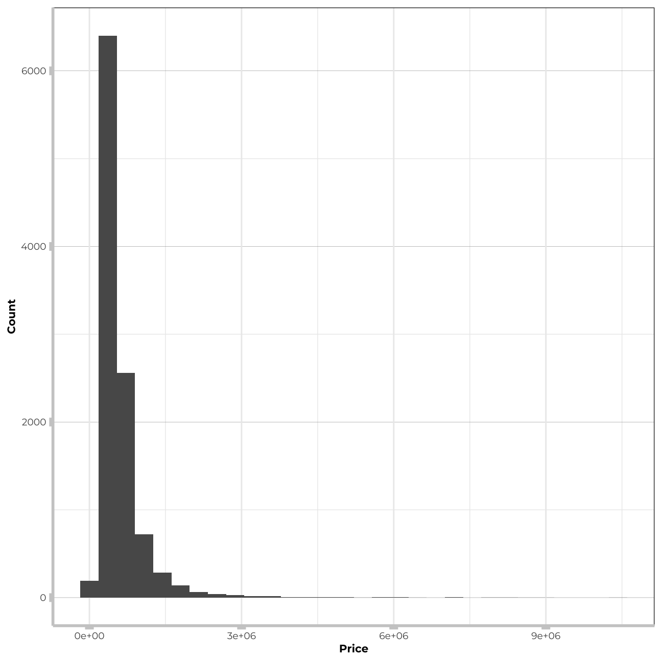
#distirbution of log price
train_data %>%
  ggplot(aes(x=log(price)))+
  geom_histogram()+
  theme_bw() +
  theme(panel.grid.major.y = element_line(color = "gray60", size = 0.1),
        panel.background = element_rect(fill = "white", colour = "white"),
        axis.line = element_line(size = 1, colour = "grey80"),
        axis.ticks = element_line(size = 3,colour = "grey80"),
        plot.title = element_text(color = "grey80",size=15,face="bold", family= "Montserrat"),
        axis.title.y = element_text(size = 8, angle = 90, family="Montserrat", face = "bold"),
        axis.text.y=element_text(family="Montserrat", size=7),
        axis.title.x = element_text(size = 8, family="Montserrat", face = "bold"),
        axis.text.x=element_text(family="Montserrat", size=7))+
    labs(x="Log Price", y="Count")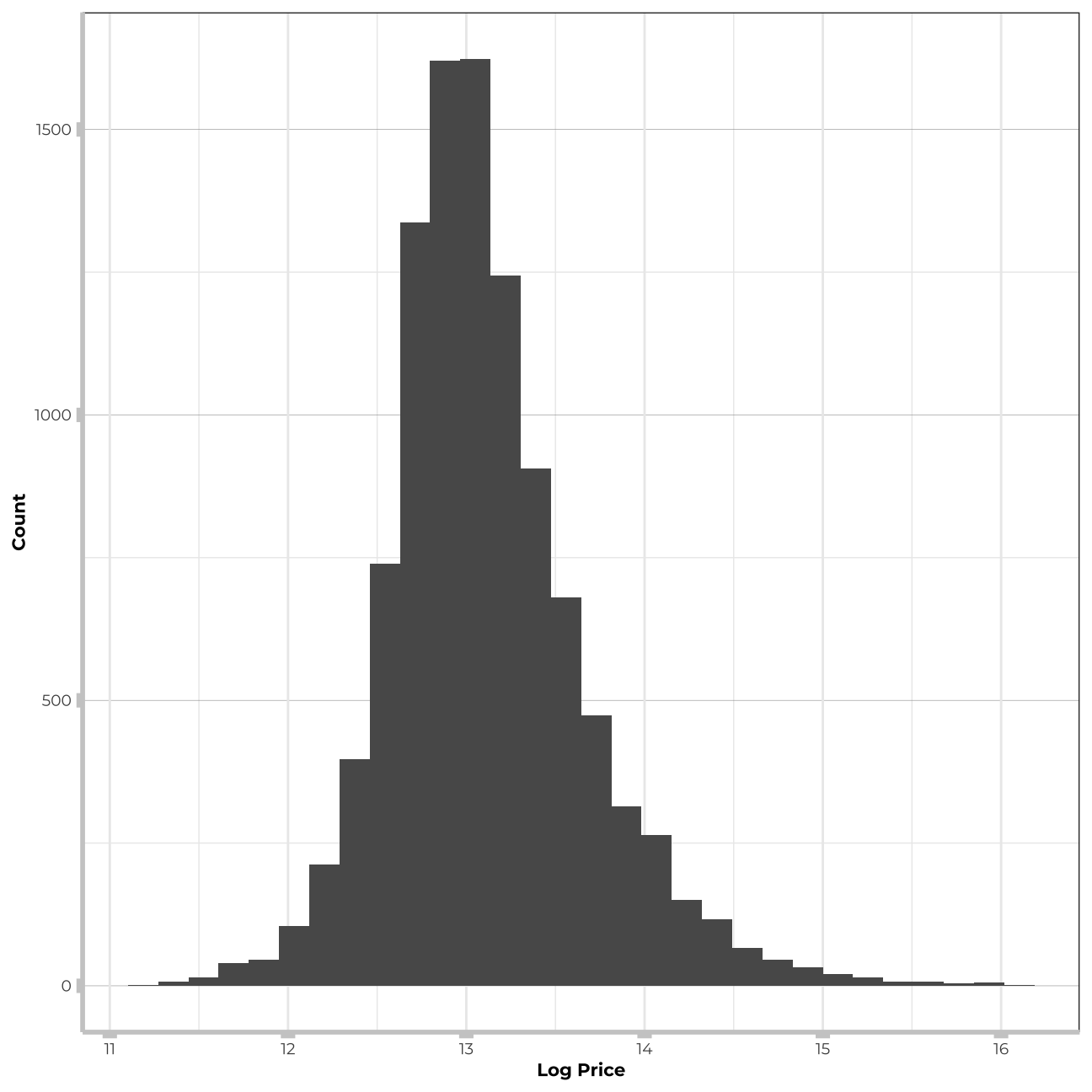
#train_data_log <- train_data %>%
#  mutate(log_price=log(price))
Price variable is highly right-skewed. For sake of this exercise I will not run the algorithm on the log price as the stack algorithm can use only one dependent variable. Tree based models that I will build in further steps can handle such a distribution much better and possibly will perform even better for price than for log(price). Therefore, to stay consistent, I will stick to “price” for all my models.
Numeric variables
I will now estimate a correlation table between prices and other continuous variables.
# produce a correlation table using GGally::ggcor()
# this takes a while to plot
#let's remember these are only correlations for numeric variables - the correlations for factor data can be also strongly related, what we could observe in the graphs before
train_data %>%
select(-ID) %>% #keep Y variable last
ggcorr(method = c("pairwise", "pearson"), layout.exp = 2,label_round=2, label = TRUE,label_size = 2,hjust = 1,nbreaks = 5,size = 2,angle = -20)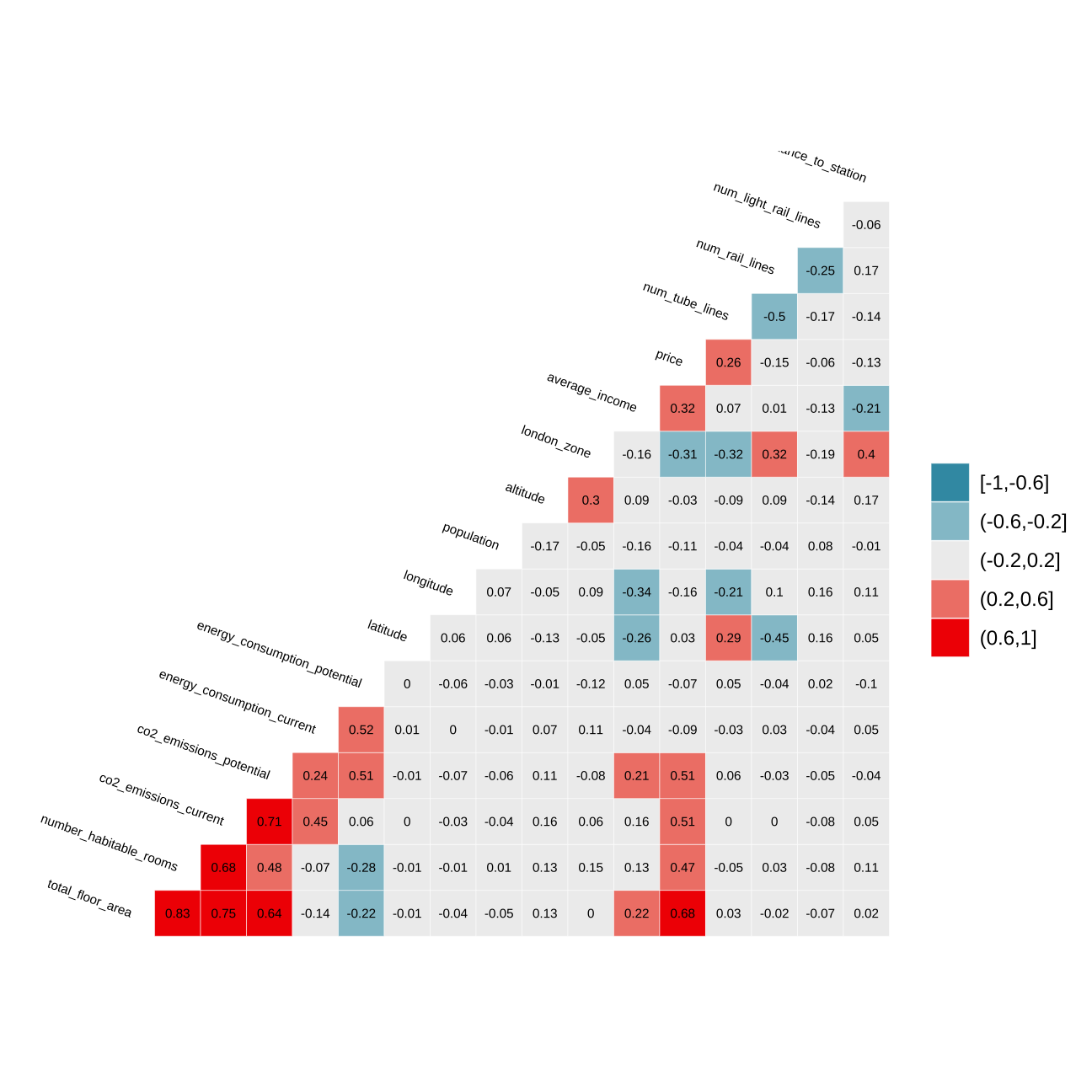 Variables that are most correlated with “price” variable are: average_income, london_zone, co2_emissions_current, co2_emissions_potential, number_habitable_rooms and total_floor_area. Nevertheless, let’s keep in mind, that pairs: co2_emissions_current & co2_emissions_potential and number_habitable_rooms & total_floor_area are highly correlated. In my models i will as well investigate interactions of variables that have a reasonable explanation and are very weakly correlated.
Fit a linear regression model
First linear model comes from the workshop. I will build on it in future models.
Model 1
# creating the control for all my future models - it needs to be the same for all of them in order to be able to stack them togehter in the end
CVfolds=15

indexProbs=createMultiFolds(train_data$price,times=1)
control <- trainControl(method = "cv", number = CVfolds, returnResamp = "final",
                     savePredictions = "final",  # needs to be final or all
                     index = indexProbs, sampling=NULL)
#we are going to train the model and report the results using k-fold cross validation
#set.seed(1)
#model1_lm<-train(
#    price ~ distance_to_station +water_company+property_type+whether_old_or_new+freehold_or_leasehold+latitude+ longitude,
#    train_data,
#   method = "lm",
#    trControl = control
#   )

# summary of the results
#summary(model1_lm)
Model 2
#we are going to train the model and report the results using k-fold cross validation
#set.seed(1)
#model2_lm<-train(
#    price ~ total_floor_area+ number_habitable_rooms+ co2_emissions_current+co2_emissions_potential +average_income+ #longitude+num_tube_lines+num_rail_lines+distance_to_station,
#    train_data,
#  method = "lm",
#    trControl = control
#   )

# summary of the results
#summary(model2_lm)
Model 3
#we are going to train the model and report the results using k-fold cross validation
#set.seed(1)
#model3_lm<-train(
#    price ~ total_floor_area+ number_habitable_rooms+ co2_emissions_potential +average_income+ longitude+num_tube_lines+property_type+current_energy_rating+windows_energy_eff +district+type_of_closest_station,
#    train_data,
#   method = "lm",
#    trControl = control
#   )

# summary of the results
#summary(model3_lm)
Model 4
#we are going to train the model and report the results using k-fold cross validation
#set.seed(1)
#model4_lm<-train(
#    price ~ poly(total_floor_area,3)+sqrt(number_habitable_rooms)+number_habitable_rooms +average_income+ #longitude+num_tube_lines+windows_energy_eff +district+type_of_closest_station+ #property_type*type_of_closest_station+london_zone*distance_to_station+london_zone*property_type,
#    train_data,
#  method = "lm",
#    trControl = control
#   )

# summary of the results
#summary(model4_lm)
Model 5 - Final model
In this model, I will add all the significant interactions that I found and the postcode_short variable.
#we are going to train the model and report the results using k-fold cross validation
set.seed(1)
model5_lm<-train(
    price ~ poly(total_floor_area,3)+number_habitable_rooms+sqrt(number_habitable_rooms)+average_income+current_energy_rating+windows_energy_eff+ property_type*type_of_closest_station+london_zone*distance_to_station+water_company+num_tube_lines+is_station+total_floor_area:london_zone+total_floor_area:num_tube_lines+average_income:number_habitable_rooms+postcode_short+district,
    train_data,
   method = "lm",
    trControl = control)
# summary of the results
# summary(model5_lm)
## ---
## Signif. codes: 0 '***' 0.001 '**' 0.01 '*' 0.05 '.' 0.1 ' ' 1
##
## Residual standard error: 213000 on 10216 degrees of freedom
## Multiple R-squared: 0.839, Adjusted R-squared: 0.834
## F-statistic: 188 on 282 and 10216 DF, p-value: <2e-16performancelr<- list()
performancelr[2]<- model5_lm[[4]] %>%
select(RMSE) %>%
pull()
performancelr[1]<- model5_lm[[4]] %>%
select(Rsquared) %>%
pull()
names(performancelr) <- c("Rsquare", "RMSE")
performancelr## $Rsquare
## [1] 0.82
##
## $RMSE
## [1] 222161Model log
I will now try out how well the log_price performs vs. the unlogged one
Importance
# we can check variable importance as well
#importance1 <- varImp(model1_lm, scale=TRUE)
#plot(importance1)

#importance2 <- varImp(model2_lm, scale=TRUE)
#plot(importance2)

#importance3 <- varImp(model3_lm, scale=TRUE)
#plot(importance3)

#importance4 <- varImp(model4_lm, scale=TRUE)
#plot(importance4)

importance5<- varImp(model5_lm, scale=TRUE)
plot(importance5)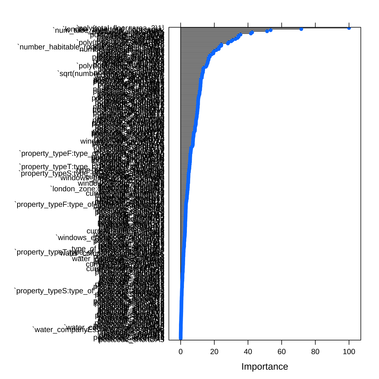
#importance5_log<- varImp(model5_lm_log, scale=TRUE)
#plot(importance5_log)
Predict the values in testing and out of sample data
Below I use the predict function to test the performance of the model in testing data and summarize the performance of the linear regression model. I can measure the quality of my predictions when looking at vlaues of RMSE and Rsquare. The lower the RMSE, the lower the error we can get in our predicted data. The higher the Rsquared, the more percentage of data is explained by the model.
# We can predict the testing values

#prediting the results on test_data
set.seed(1)
predictions <- predict(model5_lm,test_data)
summary(predictions)
## Min. 1st Qu. Median Mean 3rd Qu. Max.
## -186064 351066 463098 590293 653951 8552732summary(train_data$price) # checking if the values are similar to the true ones## Min. 1st Qu. Median Mean 3rd Qu. Max.
## 77000 350000 460000 594480 655000 10500000lr_results<-data.frame( RMSE = RMSE(predictions, test_data$price),
Rsquare = R2(predictions, test_data$price))
lr_results ## RMSE Rsquare
## 1 202699 0.842#We can predict prices for out of sample data the same way
#predictions_oos <- predict(model5_lm,london_house_prices_2019_out_of_sample)
#predictions_oosTree model
Next I fit a tree model using the same subset of features. Again I will add more variables in the next steps and tune the parameter of my tree to find a better fit.
First model
#model2_tree <- train(
#  price ~ distance_to_station +water_company+property_type+whether_old_or_new+freehold_or_leasehold+latitude+ longitude,
#  train_data,
#  method = "rpart",
#  trControl = control,
#  tuneLength=2
#    )

#You can view how the tree performs
#model2_tree$results

#You can view the final tree
#rpart.plot(model2_tree$finalModel)

#you can also visualize the variable importance
#importance <- varImp(model2_tree, scale=TRUE)
#plot(importance)
Model tree 2
#model3_tree <- train(
#  price ~ total_floor_area +average_income+ longitude+num_tube_lines #+property_type+london_zone+distance_to_station+latitude+is_station+number_habitable_rooms+current_energy_rating+windows_energy_eff+ #is_district,
#  train_data,
#  method = "rpart",
#  trControl = control,
#  tuneLength=15
# )


#You can view how the tree performs
#model3_tree$results

#You can view the final tree
#rpart.plot(model3_tree$finalModel)

#you can also visualize the variable importance
#importance <- varImp(model3_tree, scale=TRUE)
#plot(importance)
#importance
Tree model 4
#set.seed(1)
#model4_tree <- train(
#  price ~ total_floor_area +average_income+ longitude+latitude+
#    num_tube_lines +
#    property_type+london_zone+distance_to_station+is_station+is_district+current_energy_rating+type_of_closest_station,
#  train_data,
#  method = "rpart",
#  trControl = control,
#  tuneLength=15
#    )

#You can view how the tree performs
#model4_tree$results

#You can view the final tree
#rpart.plot(model4_tree$finalModel)

#you can also visualize the variable importance
#importance <- varImp(model4_tree, scale=TRUE)
#plot(importance)

#varImp(model4_tree)
Next tree model
#setting seed
set.seed(1)
#prediction for next model
modeltrial2 <- train(
  price ~ total_floor_area +average_income+ longitude+latitude+current_energy_rating+num_tube_lines +type_of_closest_station+property_type+london_zone+distance_to_station+is_station+is_district+is_postcode,
  train_data,
  method = "rpart",
  metric="Rsquared",
 trControl = control,
  tuneLength=15)

# performance of the tree
modeltrial2$results
## cp RMSE Rsquared MAE RMSESD RsquaredSD MAESD
## 1 0.00678 280228 0.711 158448 28626 0.0613 4687
## 2 0.00857 286345 0.697 163129 33236 0.0657 4141
## 3 0.00891 288773 0.692 165861 33296 0.0671 5390
## 4 0.00904 289539 0.690 166786 32845 0.0660 5116
## 5 0.00988 290066 0.689 167704 33655 0.0680 6222
## 6 0.01043 291305 0.686 169564 32881 0.0691 6875
## 7 0.01117 295575 0.677 172553 32559 0.0659 6828
## 8 0.01330 299305 0.668 174214 33552 0.0758 7039
## 9 0.01519 307410 0.650 178251 36428 0.0774 5840
## 10 0.03224 322109 0.620 181936 40114 0.0658 7637
## 11 0.03852 332548 0.598 184410 47044 0.0799 9421
## 12 0.04310 346772 0.558 194132 41461 0.0729 9683
## 13 0.07590 369473 0.495 214703 42384 0.0995 15876
## 14 0.16197 424347 0.343 235566 57846 0.0698 10491
## 15 0.31416 470699 0.294 257490 50547 0.0316 22986# view the final tree
rpart.plot(modeltrial2$finalModel)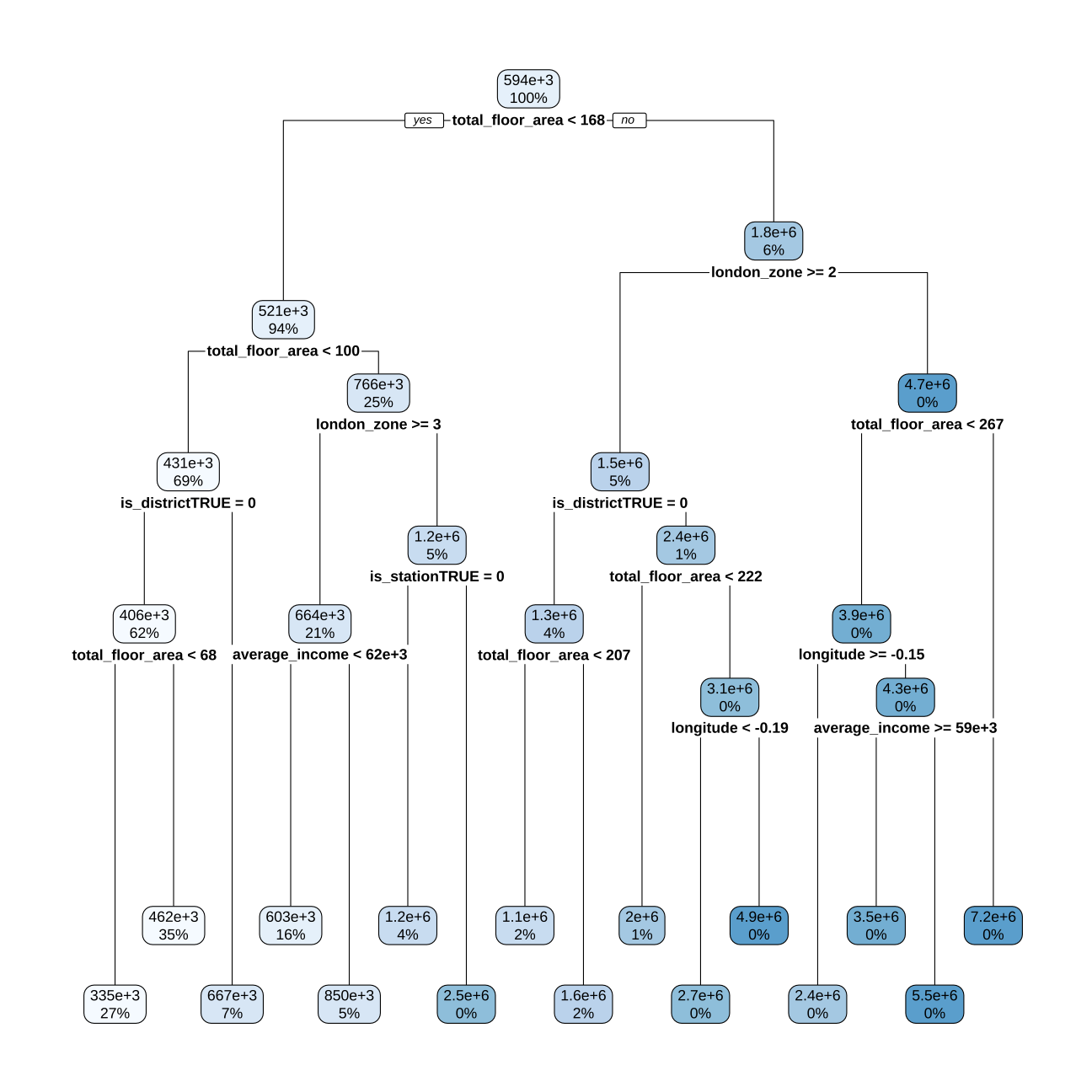
# you can also visualize the variable importance
#importance <- varImp(modeltrial2, scale=TRUE)
#plot(importance)

#varImp(modeltrial2)
Choosing the right split for model tree 4
#modelLookup("rpart")

#I choose cp values that seems to result in low error based on plot above
Grid <- expand.grid(cp = seq( 0.000, 0.00085,0.00005))


#choosing seed
set.seed(1)
#training model
modeltrial2 <- train(
  price ~ total_floor_area +average_income+ longitude+latitude+current_energy_rating+num_tube_lines +type_of_closest_station+property_type+london_zone+distance_to_station+postcode_short+district+energy_consumption_current+is_station+is_district+is_postcode,
  train_data,
  method = "rpart",
  metric="Rsquared",
  trControl = control,
  tuneGrid=Grid)


#performance of the model
print(modeltrial2)
## CART
##
## 10499 samples
## 16 predictor
##
## No pre-processing
## Resampling: Cross-Validated (15 fold)
## Summary of sample sizes: 9449, 9450, 9449, 9449, 9448, 9450, ...
## Resampling results across tuning parameters:
##
## cp RMSE Rsquared MAE
## 0.00000 238948 0.792 116769
## 0.00005 238798 0.792 116161
## 0.00010 239072 0.791 117372
## 0.00015 240248 0.789 119481
## 0.00020 240670 0.788 120771
## 0.00025 241638 0.786 121826
## 0.00030 241753 0.786 122536
## 0.00035 242028 0.785 123863
## 0.00040 243232 0.783 124706
## 0.00045 244243 0.781 125638
## 0.00050 245215 0.779 126421
## 0.00055 245621 0.779 127182
## 0.00060 245995 0.778 127453
## 0.00065 246394 0.777 128082
## 0.00070 246982 0.776 128714
## 0.00075 247834 0.774 129626
## 0.00080 248632 0.773 130377
## 0.00085 249088 0.772 131070
##
## Rsquared was used to select the optimal model using the largest value.
## The final value used for the model was cp = 0.#plot of the cp values
plot(modeltrial2)
#plotting the tree
rpart.plot(modeltrial2$finalModel)
Final tree model
#choosing small grid so the algorithm choose the best local cp
Grid <- expand.grid(cp = seq( 0.00005, 0.00015,0.00005))

#setting seed
set.seed(1)
#training model
model_tree_final <- train(
  price ~ total_floor_area +average_income+ longitude+latitude+current_energy_rating+num_tube_lines +type_of_closest_station+property_type+london_zone+distance_to_station+postcode_short+district+energy_consumption_current+is_station+is_district+is_postcode,
  train_data,
  method = "rpart",
  metric="Rsquared",
  trControl = control,
  tuneGrid=Grid)

#plotting cp
plot(model_tree_final)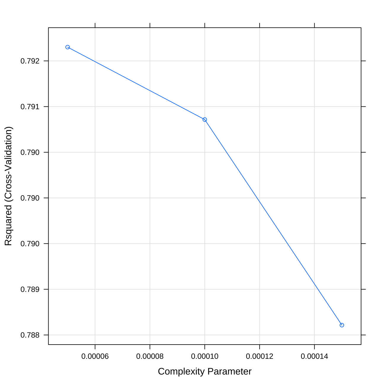
#plotting tree
rpart.plot(model_tree_final$finalModel)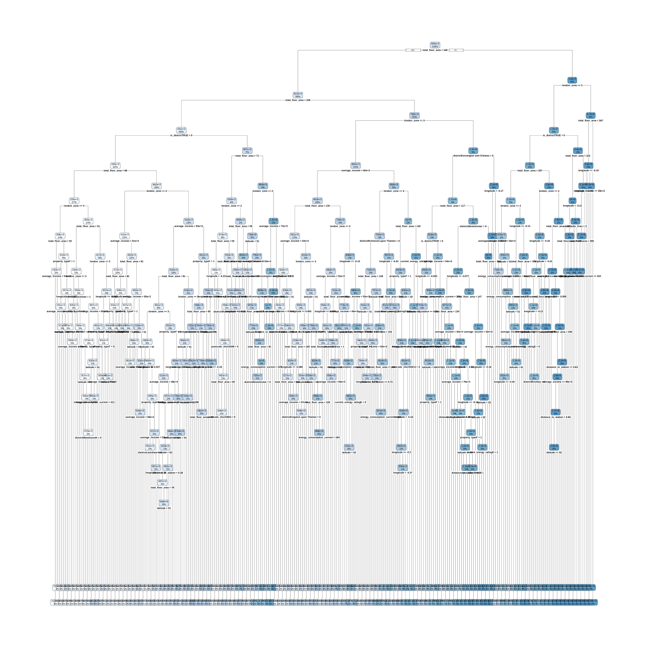
#Predict the probabilities using the tree model in testing data
predictions_tree <- predict(model_tree_final,test_data)

tree_results<-data.frame(  RMSE = RMSE(predictions_tree, test_data$price),
                            Rsquare = R2(predictions_tree, test_data$price))
tree_results
## RMSE Rsquare
## 1 242413 0.777#RMSE & Rsquare of final tree model
performancetree<- list() #creating list
performancetree[2]<- model_tree_final[[4]] %>%
filter(cp == model_tree_final$bestTune$cp) %>% #adding RMSE
select(RMSE) %>%
pull()
performancetree[1]<- model_tree_final[[4]] %>%
filter(cp == model_tree_final$bestTune$cp) %>% #adding Rsquare
select(Rsquared) %>%
pull()
names(performancetree) <- c("Rsquare", "RMSE") #rename
performancetree## $Rsquare
## [1] 0.792
##
## $RMSE
## [1] 238798As expected a single tree in this case does not perform this well, however it is expected. This is why in my further analysis I will use hundreds of trees. One single tree overfits easily and is not the best predictor.
Other algorithms
I will use three other algorithms to predict prices. I will also tune the parameters of these algorithms in order to obtain best possible performance.
LASSO model
#  LASSO model

#we will look for the optimal lambda in this sequence
lambda_seq <- seq(0, 5000, length = 1000)


#LASSO regression with using 5-fold cross validation to select the best lambda amonst the lambdas specified in "lambda_seq".
#setting seed
set.seed(1)
#training lasso model
lasso <- train(
 price~ whether_old_or_new+freehold_or_leasehold+latitude+ longitude+ poly(total_floor_area,3)+average_income+current_energy_rating+windows_energy_eff +district+ property_type*type_of_closest_station+london_zone*distance_to_station+water_company+is_station+number_habitable_rooms+sqrt(number_habitable_rooms)+ num_tube_lines+total_floor_area:london_zone+total_floor_area:num_tube_lines+average_income:number_habitable_rooms+co2_emissions_current+co2_emissions_potential+postcode_short+is_district+is_postcode,
 data = train_data,
 method = "glmnet",
  preProc = c("center", "scale"), #This option standardizes the data before running the LASSO regression
  trControl = control,
  tuneGrid = expand.grid(alpha = 1, lambda = lambda_seq) #alpha=1 specifies to run a LASSO regression. If alpha=0 the model would run ridge regression.
  )
#plotting lamba values
plot(lasso)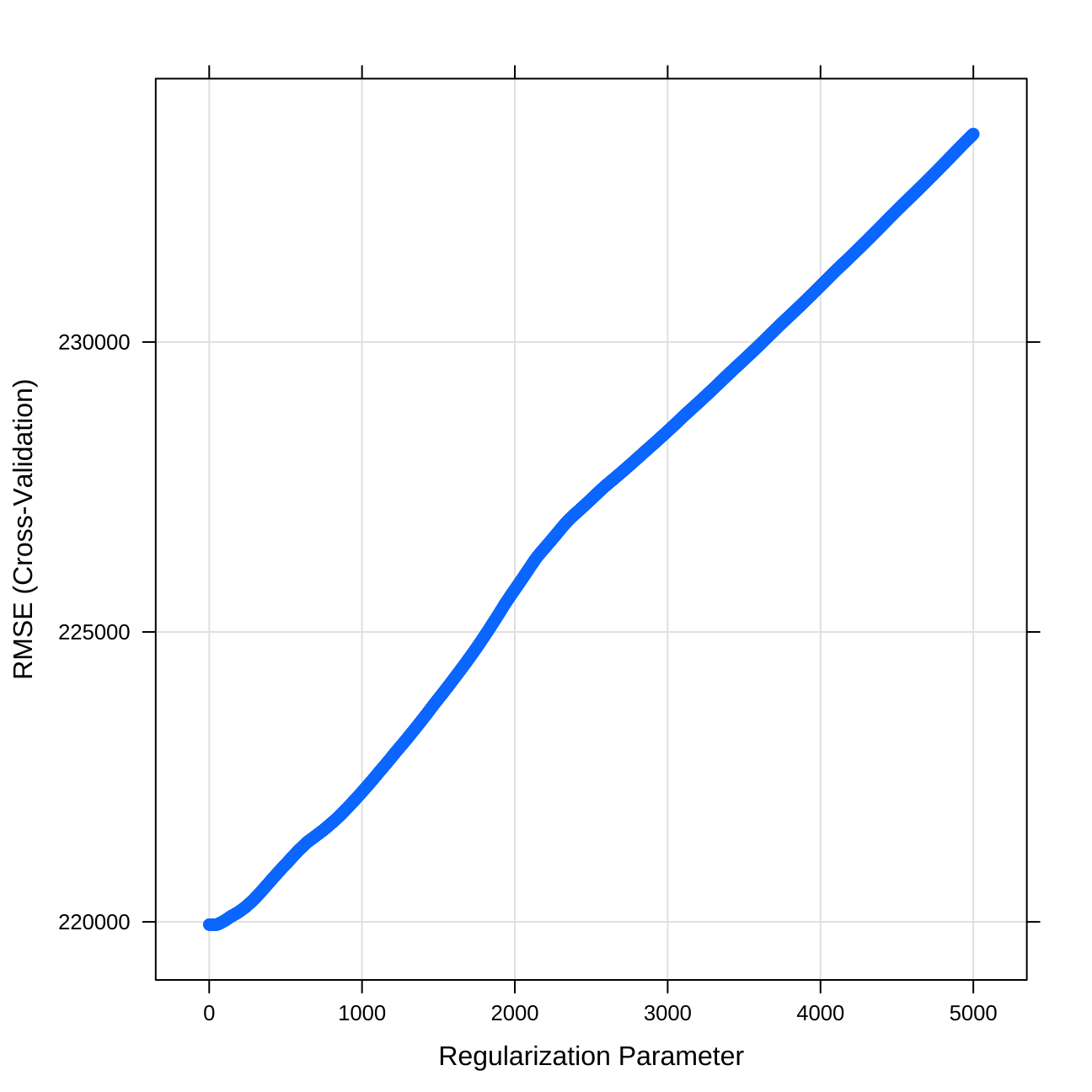
#coef(lasso$finalModel, lasso$bestTune$lambda) #best lambda

#RMSE & Rsquare of the model
performancelasso<- list() #creating a list
performancelasso[2]<- lasso[[4]] %>%  #adding RMSE
  filter(lambda == lasso$bestTune$lambda) %>%
  select(RMSE) %>%
  pull()

performancelasso[1]<- lasso[[4]] %>%  #adding Rsquare
  filter(lambda == lasso$bestTune$lambda) %>%
  select(Rsquared) %>%
  pull()

names(performancelasso) <- c("Rsquare", "RMSE") #rename
performancelasso
## $Rsquare
## [1] 0.823
##
## $RMSE
## [1] 219953#prediction on test_data
predictions_lasso <- predict(lasso,test_data)
# Model prediction performance
LASSO_results<-data.frame( RMSE = RMSE(predictions_lasso, test_data$price),
Rsquare = R2(predictions_lasso, test_data$price))
LASSO_results ## RMSE Rsquare
## 1 201073 0.844As we can see, the best performance is for lambda=0, which translates for linear regression with no regularization. Therefore, in my multimodel, I will choose only one of these.
RANDOM FOREST
Parameters for random forest models in the ranger function that implements random forest i) ‘mtry’: number of randomly chosen variables to do a split each time ii) splitrule: purity measure we use. I will only use gini iii) min.node.size: Minimum size allowed for a leaf iv) ‘importance’: is an option to get a sense of the importance of the variables. We will use it below.
modelLookup("ranger")## model parameter label forReg forClass probModel
## 1 ranger mtry #Randomly Selected Predictors TRUE TRUE TRUE
## 2 ranger splitrule Splitting Rule TRUE TRUE TRUE
## 3 ranger min.node.size Minimal Node Size TRUE TRUE TRUE# Define the tuning grid: tuneGrid
Gridtune= data.frame(mtry=c(10:15),
min.node.size = 5,
splitrule="variance")
# we will now train random forest model
#set seed
set.seed(1)
#train model
rfregFit <- train(price~poly(total_floor_area,2) +average_income+ longitude+latitude+current_energy_rating+num_tube_lines +type_of_closest_station+property_type+london_zone+distance_to_station+is_station+is_district +water_company+freehold_or_leasehold+is_postcode ,
data = train_data,
method = "ranger",
trControl=control,
# calculate importance
importance="permutation",
tuneGrid = Gridtune,
num.trees = 200)
#importance of variables
varImp(rfregFit)## ranger variable importance
##
## only 20 most important variables shown (out of 26)
##
## Overall
## poly(total_floor_area, 2)1 100.000
## poly(total_floor_area, 2)2 31.097
## london_zone 26.664
## is_districtTRUE 22.242
## longitude 15.167
## average_income 8.483
## is_stationTRUE 8.187
## freehold_or_leaseholdL 8.179
## latitude 7.732
## property_typeF 6.489
## is_postcodeTRUE 3.408
## num_tube_lines 2.732
## distance_to_station 2.241
## property_typeT 2.129
## water_companyThames Water 1.340
## type_of_closest_stationtube 1.034
## property_typeS 0.934
## type_of_closest_stationrail 0.733
## water_companyEssex & Suffolk Water 0.441
## current_energy_ratingC 0.400#plot of important variables
plot(varImp(rfregFit))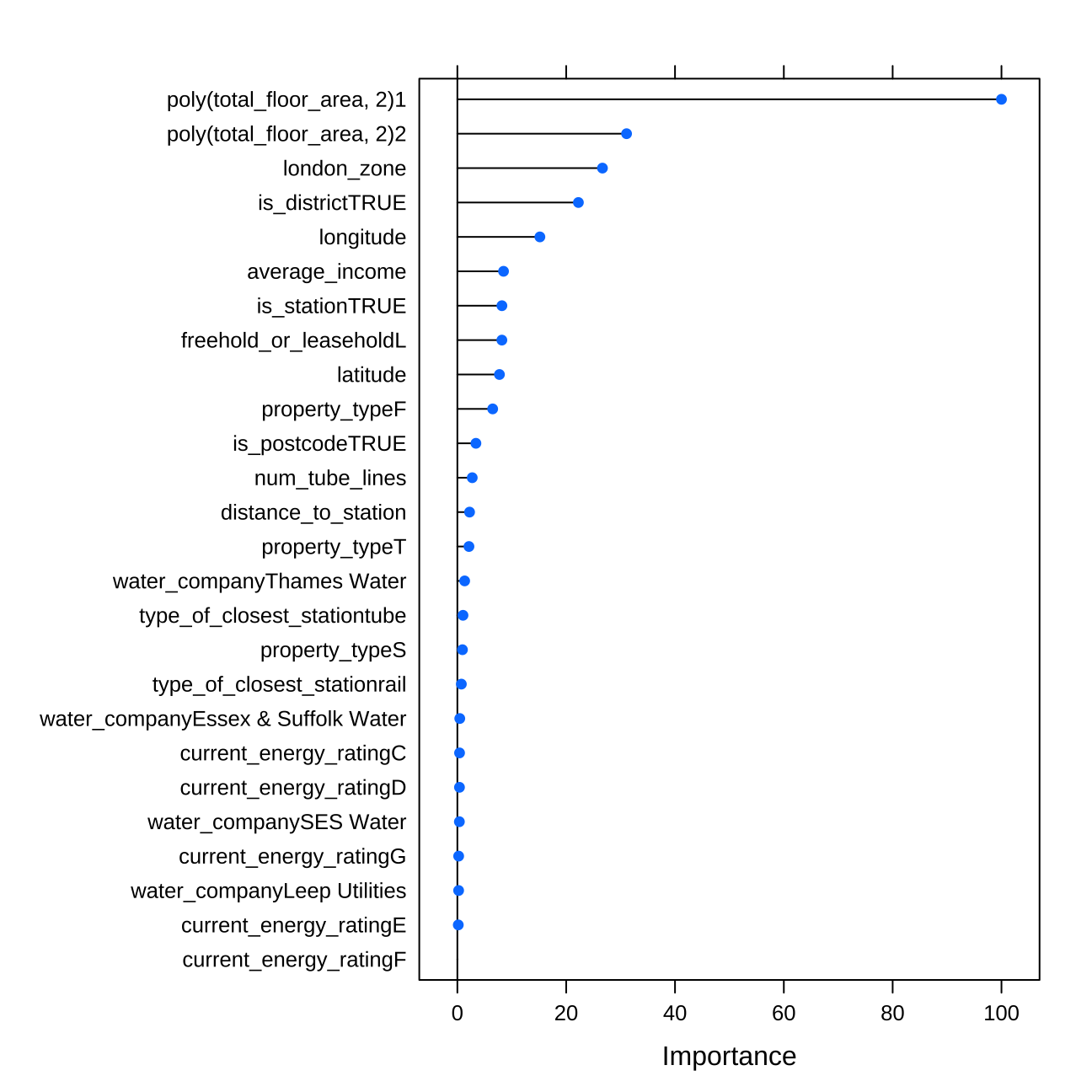
#summary of grid tuning & RMSE &Rsquare
print(rfregFit)
## Random Forest
##
## 10499 samples
## 15 predictor
##
## No pre-processing
## Resampling: Cross-Validated (15 fold)
## Summary of sample sizes: 9449, 9450, 9449, 9449, 9448, 9450, ...
## Resampling results across tuning parameters:
##
## mtry RMSE Rsquared MAE
## 10 193471 0.863 93978
## 11 194828 0.861 94385
## 12 194761 0.861 94560
## 13 194908 0.861 94448
## 14 194910 0.861 94717
## 15 195655 0.860 95110
##
## Tuning parameter 'splitrule' was held constant at a value of variance
##
## Tuning parameter 'min.node.size' was held constant at a value of 5
## RMSE was used to select the optimal model using the smallest value.
## The final values used for the model were mtry = 10, splitrule = variance
## and min.node.size = 5.#predictions for data_test
predictions_rf <-predict(rfregFit,test_data)
# Model prediction performance
rf_results<-data.frame( RMSE = RMSE(predictions_rf, test_data$price),
Rsquare = R2(predictions_rf, test_data$price))
rf_results ## RMSE Rsquare
## 1 191418 0.86GRADIENT BOOSTING MACHINE
modelLookup("gbm")## model parameter label forReg forClass probModel
## 1 gbm n.trees # Boosting Iterations TRUE TRUE TRUE
## 2 gbm interaction.depth Max Tree Depth TRUE TRUE TRUE
## 3 gbm shrinkage Shrinkage TRUE TRUE TRUE
## 4 gbm n.minobsinnode Min. Terminal Node Size TRUE TRUE TRUE#Expand the search grid (see above for definitions)
grid<-expand.grid(interaction.depth = 8,n.trees = 500,shrinkage =0.05, n.minobsinnode = 5)
#Train for gbm
#set seed
set.seed(1)
#train model
gbmFit1 <- train(price~poly(total_floor_area,3) +average_income+ longitude+latitude+current_energy_rating+num_tube_lines +property_type+london_zone*distance_to_station+is_station+is_district +water_company+freehold_or_leasehold+is_postcode+total_floor_area:london_zone+property_type:type_of_closest_station+district,
data = train_data,
method = "gbm",
trControl = control,
tuneGrid =grid,
metric = "RMSE",
verbose = FALSE
)
#RMSE & Rsquare
print(gbmFit1)## Stochastic Gradient Boosting
##
## 10499 samples
## 16 predictor
##
## No pre-processing
## Resampling: Cross-Validated (15 fold)
## Summary of sample sizes: 9449, 9450, 9449, 9449, 9448, 9450, ...
## Resampling results:
##
## RMSE Rsquared MAE
## 197973 0.856 97070
##
## Tuning parameter 'n.trees' was held constant at a value of 500
## Tuning
##
## Tuning parameter 'shrinkage' was held constant at a value of 0.05
##
## Tuning parameter 'n.minobsinnode' was held constant at a value of 5#variables importance
varImp(gbmFit1)## gbm variable importance
##
## only 20 most important variables shown (out of 67)
##
## Overall
## poly(total_floor_area, 3)1 100.000
## london_zone 29.678
## is_districtTRUE 16.556
## poly(total_floor_area, 3)2 11.677
## longitude 9.069
## districtKensington and Chelsea 8.390
## average_income 7.772
## is_stationTRUE 6.949
## london_zone:total_floor_area 5.772
## is_postcodeTRUE 4.916
## latitude 4.431
## poly(total_floor_area, 3)3 4.335
## london_zone:distance_to_station 2.795
## distance_to_station 2.380
## districtWestminster 1.383
## num_tube_lines 1.352
## property_typeF 0.998
## freehold_or_leaseholdL 0.870
## current_energy_ratingD 0.489
## property_typeT 0.344#plot on variables importance
plot(varImp(gbmFit1))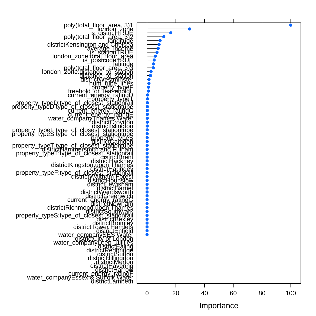
#performance of predicted values on test_data
predictions_GBM <-predict(gbmFit1, test_data)

GBM_results<-data.frame(  RMSE = RMSE(predictions_GBM, test_data$price),
                            Rsquare = R2(predictions_GBM, test_data$price))
GBM_results
## RMSE Rsquare
## 1 186632 0.866All models’ performance compared
Now I will compare performance of all my models. To do so, I will compare the Rsquare (not the Adjusted one!) of all the models.
performancelr## $Rsquare
## [1] 0.82
##
## $RMSE
## [1] 222161performancetree## $Rsquare
## [1] 0.792
##
## $RMSE
## [1] 238798performancelasso ## $Rsquare
## [1] 0.823
##
## $RMSE
## [1] 219953 print(rfregFit)## Random Forest
##
## 10499 samples
## 15 predictor
##
## No pre-processing
## Resampling: Cross-Validated (15 fold)
## Summary of sample sizes: 9449, 9450, 9449, 9449, 9448, 9450, ...
## Resampling results across tuning parameters:
##
## mtry RMSE Rsquared MAE
## 10 193471 0.863 93978
## 11 194828 0.861 94385
## 12 194761 0.861 94560
## 13 194908 0.861 94448
## 14 194910 0.861 94717
## 15 195655 0.860 95110
##
## Tuning parameter 'splitrule' was held constant at a value of variance
##
## Tuning parameter 'min.node.size' was held constant at a value of 5
## RMSE was used to select the optimal model using the smallest value.
## The final values used for the model were mtry = 10, splitrule = variance
## and min.node.size = 5.print(gbmFit1)## Stochastic Gradient Boosting
##
## 10499 samples
## 16 predictor
##
## No pre-processing
## Resampling: Cross-Validated (15 fold)
## Summary of sample sizes: 9449, 9450, 9449, 9449, 9448, 9450, ...
## Resampling results:
##
## RMSE Rsquared MAE
## 197973 0.856 97070
##
## Tuning parameter 'n.trees' was held constant at a value of 500
## Tuning
##
## Tuning parameter 'shrinkage' was held constant at a value of 0.05
##
## Tuning parameter 'n.minobsinnode' was held constant at a value of 5We can compare linear regression & LASSO model - they both perform quite similarly due to the complexity of linear regression. On the other hand, when we run the tree model, a single tree performs always much worse than more complex models - Random Forest and Gradient Boosting Machine. Nevertheless, in the stacking model, it is good to stack numerous models as they are able to catch different kinds of results. E.g. linear regression is able to catch much better the linear trends.
Stacking
I will now use stacking to ensemble 4 of my created algorithms.
multimodel<- list(tree=model_tree_final,lasso=lasso,ranger= rfregFit, gbm= gbmFit1)
class(multimodel)<- "caretList"
Visualising results
modelCor(resamples(multimodel)) #correlation matrix of the models## tree lasso ranger gbm
## tree 1.000 0.860 0.912 0.890
## lasso 0.860 1.000 0.916 0.866
## ranger 0.912 0.916 1.000 0.941
## gbm 0.890 0.866 0.941 1.000dotplot(resamples(multimodel), metric="Rsquared") #Rsquare comparison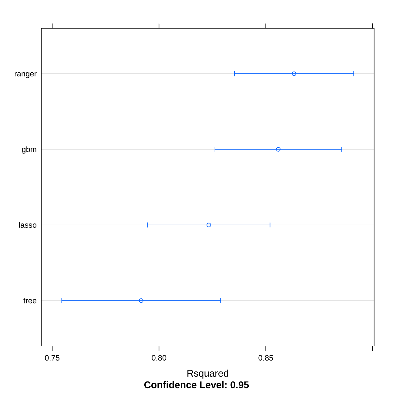
xyplot(resamples(multimodel), metric="Rsquared") #tree vs lasso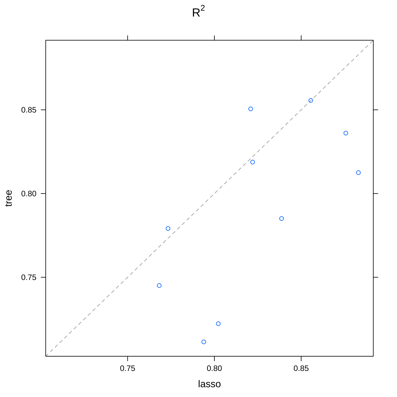
splom(resamples(multimodel), metric="Rsquared") #all the models' performance interactions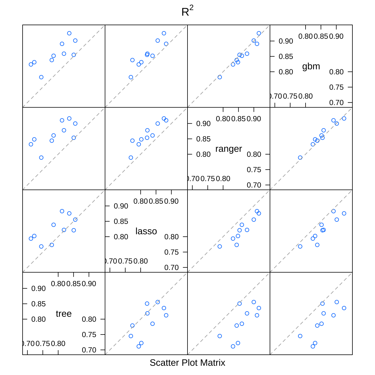
Creation of the stack model
library(caret)
library(caretEnsemble)
model_list<- caretStack(multimodel, #creating a model that stacks both models together
                        trControl=control,
                        method="lm",
                        metric="RMSE")

#summary of the model
summary(model_list)
##
## Call:
## lm(formula = .outcome ~ ., data = dat)
##
## Residuals:
## Min 1Q Median 3Q Max
## -4032689 -49841 1715 50655 4049428
##
## Coefficients:
## Estimate Std. Error t value Pr(>|t|)
## (Intercept) -2.30e+04 3.08e+03 -7.46 9.2e-14 ***
## tree 3.35e-03 1.32e-02 0.25 0.8
## lasso 2.10e-01 1.36e-02 15.45 < 2e-16 ***
## ranger 5.79e-01 2.79e-02 20.74 < 2e-16 ***
## gbm 2.45e-01 2.46e-02 9.92 < 2e-16 ***
## ---
## Signif. codes: 0 '***' 0.001 '**' 0.01 '*' 0.05 '.' 0.1 ' ' 1
##
## Residual standard error: 192000 on 10494 degrees of freedom
## Multiple R-squared: 0.865, Adjusted R-squared: 0.865
## F-statistic: 1.68e+04 on 4 and 10494 DF, p-value: <2e-16# RMSE & Rsquaere
performancefinal<- list() #creating a list
performancefinal[2]<- model_list[[3]] %>% #adding RMSE
select(RMSE) %>%
pull()
performancefinal[1]<- model_list[[3]] %>% #adding Rsquare
select(Rsquared) %>%
pull()
names(performancefinal) <- c("Rsquare", "RMSE") #rename
performancefinal #check the values## $Rsquare
## [1] 0.868
##
## $RMSE
## [1] 189661As we can see, the Rsuqared achieves the best results in comparison to our all previous models. the RMSE is equal to 189661.2 and the Rsquare equals 86.8%. Therefore, we will use this model as an estimation engine to guide the investment on the housing market in London.
Performance on test data
First I will check the preformance of our model on the test dataset.
numchoose=200 #choosing number of investments
set.seed(1) #set seed
random_mult<-1/(1-runif(nrow(test_data),min=-0.2, max=0.2))
test_data$asking_price<-test_data$price*random_mult #creating the asking_price simulation

#Assume that these are asking prices

#now predict the value of houses
test_data$predict<-predict(model_list,test_data)

#choose the ones that you want to invest here

#Let’s find the profit margin given our predicted price and asking price

test_data<-test_data %>%
  mutate(profitMargin=(predict-asking_price)/(asking_price)) %>%
  arrange(-profitMargin)
#Make sure you chooses exactly 200 of them
test_data$invest=0
test_data[1:numchoose,]$invest=1

#let's find the actual profit
test_data<-test_data %>%
  mutate(profit=(price-asking_price)/(asking_price), actualProfit=invest*profit)

mean(test_data$profit)
## [1] 0.0019sum(test_data$actualProfit)/numchoose## [1] 0.0678The silumation gives us positice results with the average profit on all the investments amouting to 0.19% and the average profit from 200 best investments equal o 6%.
Picking investment portfolio
In this section I will use the best algorithm I identified to choose 200 properties from the out of sample data. I will report 20 first raws of my original dataset with the scores.
numchoose=200 # choosing number of properties we will invest in

oos<-london_house_prices_2019_out_of_sample
#predict the value of houses
oos$predict<-predict(model_list,oos)
#Choose the ones you want to invest here
#Make sure you choose exactly 200 of them

oos<-oos %>%
  mutate(profitMargin=(predict-asking_price)/(asking_price)) %>%
  arrange(-profitMargin)
#Make sure you chooses exactly 200 of them
oos$buy=0
oos[1:numchoose,]$buy=1
oos<-oos %>% mutate( actualProfit=buy*profitMargin)
#let's find the actual profit
mean(oos$profitMargin)
## [1] 0.0387sum(oos$actualProfit)/numchoose## [1] 0.685Final perdictions lead us to the following results. The average profit margin of all the properties in the data set equals 3.86%, whereas the average profit from 200 best investments equals 68.45%. Our engine works. I will provide the documentation of all the steps taken and explanantion of all the models in my technial report.
Thank you.
