Cars clustering using dimension reduction methods - PCA and LDA

PART 1: PRINCIPAL COMPONENT ANALYSIS

I am going to analyse a D = 11 data set called ‘mtcars’ which comes with R distribution. The data was extracted from the 1974 Motor Trend US magazine, and comprises fuel consumption and 10 aspects of automobile design and performance for 32 automobiles (1973–74 models).

The features of this data set are:

mpg Miles/(US) gallon
cyl Number of cylinders
disp Displacement (cu.in.)
hp Gross horsepower
drat Rear axle ratio
wt Weight (1000 lbs)
qsec 1/4 mile time
vs Engine (0 = V-shaped, 1 = straight)
am Transmission (0 = automatic, 1 = manual)
gear Number of forward gears
carb Number of carburetors

Data loading and initial analysis

In this point I will:

Load and attach the “mtcars” data to the current session.
Display the dataset and observe the inputs.

#Load data
data(mtcars)
attach(mtcars)

#View the dataframe
print(mtcars)

##                      mpg cyl  disp  hp drat   wt qsec vs am gear carb
## Mazda RX4           21.0   6 160.0 110 3.90 2.62 16.5  0  1    4    4
## Mazda RX4 Wag       21.0   6 160.0 110 3.90 2.88 17.0  0  1    4    4
## Datsun 710          22.8   4 108.0  93 3.85 2.32 18.6  1  1    4    1
## Hornet 4 Drive      21.4   6 258.0 110 3.08 3.21 19.4  1  0    3    1
## Hornet Sportabout   18.7   8 360.0 175 3.15 3.44 17.0  0  0    3    2
## Valiant             18.1   6 225.0 105 2.76 3.46 20.2  1  0    3    1
## Duster 360          14.3   8 360.0 245 3.21 3.57 15.8  0  0    3    4
## Merc 240D           24.4   4 146.7  62 3.69 3.19 20.0  1  0    4    2
## Merc 230            22.8   4 140.8  95 3.92 3.15 22.9  1  0    4    2
## Merc 280            19.2   6 167.6 123 3.92 3.44 18.3  1  0    4    4
## Merc 280C           17.8   6 167.6 123 3.92 3.44 18.9  1  0    4    4
## Merc 450SE          16.4   8 275.8 180 3.07 4.07 17.4  0  0    3    3
## Merc 450SL          17.3   8 275.8 180 3.07 3.73 17.6  0  0    3    3
## Merc 450SLC         15.2   8 275.8 180 3.07 3.78 18.0  0  0    3    3
## Cadillac Fleetwood  10.4   8 472.0 205 2.93 5.25 18.0  0  0    3    4
## Lincoln Continental 10.4   8 460.0 215 3.00 5.42 17.8  0  0    3    4
## Chrysler Imperial   14.7   8 440.0 230 3.23 5.34 17.4  0  0    3    4
## Fiat 128            32.4   4  78.7  66 4.08 2.20 19.5  1  1    4    1
## Honda Civic         30.4   4  75.7  52 4.93 1.61 18.5  1  1    4    2
## Toyota Corolla      33.9   4  71.1  65 4.22 1.83 19.9  1  1    4    1
## Toyota Corona       21.5   4 120.1  97 3.70 2.46 20.0  1  0    3    1
## Dodge Challenger    15.5   8 318.0 150 2.76 3.52 16.9  0  0    3    2
## AMC Javelin         15.2   8 304.0 150 3.15 3.44 17.3  0  0    3    2
## Camaro Z28          13.3   8 350.0 245 3.73 3.84 15.4  0  0    3    4
## Pontiac Firebird    19.2   8 400.0 175 3.08 3.85 17.1  0  0    3    2
## Fiat X1-9           27.3   4  79.0  66 4.08 1.94 18.9  1  1    4    1
## Porsche 914-2       26.0   4 120.3  91 4.43 2.14 16.7  0  1    5    2
## Lotus Europa        30.4   4  95.1 113 3.77 1.51 16.9  1  1    5    2
## Ford Pantera L      15.8   8 351.0 264 4.22 3.17 14.5  0  1    5    4
## Ferrari Dino        19.7   6 145.0 175 3.62 2.77 15.5  0  1    5    6
## Maserati Bora       15.0   8 301.0 335 3.54 3.57 14.6  0  1    5    8
## Volvo 142E          21.4   4 121.0 109 4.11 2.78 18.6  1  1    4    2

Which variables are binary in the mtcars dataset>

ANSWER: Variables ‘vs’ and ‘am’ are binary. “vs” stand for type of engine (0 = V-shaped, 1 = straight) while ‘am’ stands for transmission type (0 = automatic, 1 = manual). I will delete them later from my dataframe as the PCA works best for variables that are numeric.

What are the Dataset Requirements for PCA?

ANSWER: The Principle Component Analysis works best on the data that is as follows: - numeric data (non binary one), - correlated data - standardised: - centered in order to avoid instability - scaled ( if variables are in deifferent units)

Data pre-processing

Now I will carefully consider which variables should form inputs into the PCA model, given the numerical data requirements such that PCA works best. I will create a data frame called $\mathbb{X}$ which will contain all columns except the binary ones.

I will also: - Find the dimensionality of $\mathbb{X}$ and assign it to variable dims. - Find how many features should I be working on which are relevant for the purposes of dimensionality reduction. - Assign number of observations to variable N and number of features to variable D - Perform necessary analysis in order to establish whether the data needs centering and/or scaling.

#PCA works best for variables that are numeric. Therefore I will delete from the dataset the binary varaibles - 'vs' and 'am'
X <- data.frame()
X=mtcars %>% dplyr::select(-c(vs,am))

#Obtain dims
dims <- dim(X)
dims

## [1] 32  9

#[1] 32  9

N <- dims[[1]]  # number of observations
D <- dims[[2]]  # number of features 

# Correlation matrix dimensionality to determine if the data needs to be standardised
cov_data <- cov(X)
print(cov_data)

##          mpg     cyl    disp      hp     drat      wt     qsec    gear    carb
## mpg    36.32  -9.172  -633.1 -320.73   2.1951  -5.117   4.5091   2.136 -5.3631
## cyl    -9.17   3.190   199.7  101.93  -0.6684   1.367  -1.8869  -0.649  1.5202
## disp -633.10 199.660 15360.8 6721.16 -47.0640 107.684 -96.0517 -50.803 79.0687
## hp   -320.73 101.931  6721.2 4700.87 -16.4511  44.193 -86.7701  -6.359 83.0363
## drat    2.20  -0.668   -47.1  -16.45   0.2859  -0.373   0.0871   0.276 -0.0784
## wt     -5.12   1.367   107.7   44.19  -0.3727   0.957  -0.3055  -0.421  0.6758
## qsec    4.51  -1.887   -96.1  -86.77   0.0871  -0.305   3.1932  -0.280 -1.8941
## gear    2.14  -0.649   -50.8   -6.36   0.2760  -0.421  -0.2804   0.544  0.3266
## carb   -5.36   1.520    79.1   83.04  -0.0784   0.676  -1.8941   0.327  2.6089

cor_data <- cor(X)
print(cor_data)

##         mpg    cyl   disp     hp    drat     wt    qsec   gear    carb
## mpg   1.000 -0.852 -0.848 -0.776  0.6812 -0.868  0.4187  0.480 -0.5509
## cyl  -0.852  1.000  0.902  0.832 -0.6999  0.782 -0.5912 -0.493  0.5270
## disp -0.848  0.902  1.000  0.791 -0.7102  0.888 -0.4337 -0.556  0.3950
## hp   -0.776  0.832  0.791  1.000 -0.4488  0.659 -0.7082 -0.126  0.7498
## drat  0.681 -0.700 -0.710 -0.449  1.0000 -0.712  0.0912  0.700 -0.0908
## wt   -0.868  0.782  0.888  0.659 -0.7124  1.000 -0.1747 -0.583  0.4276
## qsec  0.419 -0.591 -0.434 -0.708  0.0912 -0.175  1.0000 -0.213 -0.6562
## gear  0.480 -0.493 -0.556 -0.126  0.6996 -0.583 -0.2127  1.000  0.2741
## carb -0.551  0.527  0.395  0.750 -0.0908  0.428 -0.6562  0.274  1.0000

SUMMARY

The data usually needs centering to ensure the numerical stability of the PCA algorithm. Therefore I will set later the “center=True” parameter when scaling.

The Variances of variables (the ones on the diagonal) are very different in scale. That suggests that the data has different units. Therefore it is necessary to scale mtcars data in such a situation. Also, we can notice directly from the data frame that the variables are delivered in different units such as miles/gallon, weight in 1000lbsl qsec (time) .

PCA Analysis

PCA Analysis - Theoretical Part

I will now give a definition of what Principal Component Analysis is and whether it is a supervised or unsupervised technique & explain what supervised and unsupervised means in the context of Machine Learning.

ANSWER: The Principal Component Analysis is a method of dimension reduction by linear transformation of variables, with the final outcome of smaller dataset, that still containts the majority (aim 60-80%) of information from the orginal large dataset. PCA is an unsupervised technique. It means that the method has no teacher signal and does not use an algorithm with any labels. Instead due to the dimension reduction it uses the principle components to come up with the final solution.

What orthogonality means when it comes to random variables being interpreted geometrically.

ANSWER: Ortogonality in this context means that the variables are not correlated with each other. It guarantees that they retain the maximum amount of variance of the dataset, which translates to explaining more variables (particularly more than 1, explained below).These orthogonal variables create na new space with less dimensions where the original, yet now uncorrelated, dataset will be represented.

I will now provide the key formula (using linear algebra notation) which allows to find the projection of vector $\mathbb{x}_n \in R^{D}$ onto M-dimensional sub-space U.

ANSWER:

$\tilde {\mathbb{x}}_n = \sum\limits_{i=1}^\mathbb{M}\mathbb{b}_iz_{ni} = \mathbb{B}\mathbb{z} =\mathbb{B}\mathbb{B}^T\mathbb{x}_n$

Where: $\tilde {\mathbb{x}}_n$ - projected vector in $R^{D}$ space

$\mathbb{b}_i$ - Principal Component Loading Vector / Basis Vector / Eigenvector” $\in R^{D}$

$z_{ni}$ - “Principal Component Score / Coordinates” $\in R^{M}$ (scalar)

Is it correct to say that covariance matrix plays key part in PCA?

ANSWER: The covariance matrix S indeed plays the crucial role in the Principal Component Analysis. It is because we aim to minimise the average squared reconstruction error. The optimisation leads to an eigenvalues problem, the solution of which we can find as follows: The eigenvectors of the covariance matrix S determine the directions of the new feature space (i.e. eigenvectors form the axes in the sub-space). The eigenvalues of the covariance matrix S explain the variance of data along the new feature axes (i.e. represent the projections of variance of data).

The crucial expression that forms a crucial part of the PCA is as follows:

$𝓙=\frac1{N}\sum\limits_{n=1}^\mathbb{N}||\mathbb{x}_n-\tilde {\mathbb{x}}_n||=\sum\limits_{j=M+1}^\mathbb{D}\mathbb{b}^T_j(\frac1{N}\sum\limits_{n=1}^\mathbb{N}\mathbb{x}_n\mathbb{x}_n^T)\mathbb{b}_j$

Where $\frac1{N}\sum\limits_{n=1}^\mathbb{N}\mathbb{x}_n\mathbb{x}_n^T$ is the Data Covariance Martix S

How the directions of the first and second principal components (basis vectors) are chosen?

ANSWER: The directions of the first and second principal components are chosen using the Data Covariance Matrix S that returns the eigenvectors (called Principal Component Loadings or PCs). They are ordered by the amount variance their correspoing eigenvalues explain in an descending order. The PCs are stored in the PCA model. They give directions of the new axes (the rotation). These are chosen by the most respective varianance of data.

i will list 4 purposes for which PCA can be used on data? Provide an explanation of what each one means.

ANSWER: The PCA can be used for the following purposes: a) data visualition - PCA enables plotting data in a 2dimensional space (called principle compenent space) through dimension reduction. The visualisation with fewer dimension becomes much more meaningful.

data compression - PCA helps in reduction of storage requirements of data what speeds up the learning algorithms substantially. It is especially useful in the era of big Data that is sometimes impossible to be processed in a reasonable amount of time.
feature extraction - PCA keeps only the important ones in order to approximate data to the desired level and removes the rest that is less meaninful. Instead of choosing features for regression or clustering, we can run PCA on our data and and obtain points projected in the new space and use the obtained result as an input to these algorithms.
noise filtering - PCA can help reduce noice in the data e.g. in speach de-noising or image de-noising.

PCA Analysis - Practical Part.

I will perform a PCA analysis on the data I called $\mathbb{X}$ above and store result into variable $\texttt{pca}$. As the data required centering and/or scaling, I will do so using optional arguments of the $\texttt{prcomp()}$ function.

#Standardise the data using prcomp
pca <- prcomp(X, center = TRUE, scale. = TRUE) 
typeof(pca) # resulting object is a list (containing 5 elements)

## [1] "list"

I use function structure, $\texttt{str()}$, to look inside my object.

#Looking inside the data
str(pca)

## List of 5
##  $ sdev    : num [1:9] 2.378 1.443 0.71 0.515 0.428 ...
##  $ rotation: num [1:9, 1:9] -0.393 0.403 0.397 0.367 -0.312 ...
##   ..- attr(*, "dimnames")=List of 2
##   .. ..$ : chr [1:9] "mpg" "cyl" "disp" "hp" ...
##   .. ..$ : chr [1:9] "PC1" "PC2" "PC3" "PC4" ...
##  $ center  : Named num [1:9] 20.09 6.19 230.72 146.69 3.6 ...
##   ..- attr(*, "names")= chr [1:9] "mpg" "cyl" "disp" "hp" ...
##  $ scale   : Named num [1:9] 6.027 1.786 123.939 68.563 0.535 ...
##   ..- attr(*, "names")= chr [1:9] "mpg" "cyl" "disp" "hp" ...
##  $ x       : num [1:32, 1:9] -0.664 -0.637 -2.3 -0.215 1.587 ...
##   ..- attr(*, "dimnames")=List of 2
##   .. ..$ : chr [1:32] "Mazda RX4" "Mazda RX4 Wag" "Datsun 710" "Hornet 4 Drive" ...
##   .. ..$ : chr [1:9] "PC1" "PC2" "PC3" "PC4" ...
##  - attr(*, "class")= chr "prcomp"

I will create 2 variables: loadings and scores, into which I store -loadings and -scores (i.e. the basis vectors and z pointing in the positive direction).

#Create load
#Loadings are the basis vectors / eigenvectors / PCs (matrix DxD) - they take name "rotation" in our data set
#I will use minus in order to provide more intuitive position direction pointing vectors
loadings<- - pca$rotation
loadings

##         PC1     PC2     PC3      PC4    PC5     PC6     PC7     PC8     PC9
## mpg   0.393 -0.0275  0.2212  0.00613  0.321 -0.7202  0.3814  0.1247 -0.1149
## cyl  -0.403 -0.0157  0.2523 -0.04070 -0.117 -0.2243  0.1589 -0.8103 -0.1627
## disp -0.397  0.0889  0.0783 -0.33949  0.487  0.0197  0.1823  0.0642  0.6619
## hp   -0.367 -0.2694  0.0172 -0.06830  0.295 -0.3539 -0.6962  0.1657 -0.2518
## drat  0.312 -0.3417 -0.1500 -0.84566 -0.162  0.0154 -0.0477 -0.1351 -0.0381
## wt   -0.373  0.1719 -0.4537 -0.19126  0.187  0.0838  0.4278  0.1984 -0.5692
## qsec  0.224  0.4840 -0.6281  0.03033  0.148 -0.2575 -0.2762 -0.3561  0.1687
## gear  0.209 -0.5508 -0.2066  0.28238  0.562  0.3230  0.0856 -0.3164 -0.0472
## carb -0.245 -0.4843 -0.4641  0.21449 -0.400 -0.3571  0.2060  0.1083  0.3205

#Create scores
#Scores are the rotated data coordinates (again I need to reverse the sign)
scores <- - pca$x 
scores

##                         PC1    PC2     PC3     PC4     PC5     PC6     PC7
## Mazda RX4            0.6642 -1.173  0.2043  0.1260 -0.7520  0.1251  0.4236
## Mazda RX4 Wag        0.6372 -0.977 -0.1108  0.0857 -0.6567  0.0662  0.4485
## Datsun 710           2.2997  0.327  0.2101  0.1086  0.0762  0.5669 -0.3861
## Hornet 4 Drive       0.2153  1.977  0.3295  0.3081  0.2439 -0.0838 -0.0330
## Hornet Sportabout   -1.5870  0.829  1.0330 -0.1474  0.2227 -0.1828  0.0579
## Valiant             -0.0496  2.447 -0.1118  0.8715  0.1257  0.2304 -0.2245
## Duster 360          -2.7144 -0.361  0.6521 -0.0963 -0.2967 -0.2776 -0.4423
## Merc 240D            2.0437  0.801 -0.8490  0.2745  0.2631  0.1904  0.3942
## Merc 230             2.2951  1.306 -1.9685 -0.0506  0.4599 -0.2044 -0.5371
## Merc 280             0.3825 -0.581 -0.8863 -0.0703 -0.4584  0.0798  0.2611
## Merc 280C            0.3665 -0.412 -1.1486 -0.0615 -0.4831  0.1607  0.0798
## Merc 450SE          -1.8847  0.724  0.2060  0.2186 -0.2800 -0.1714  0.0891
## Merc 450SL          -1.6711  0.714  0.3264  0.2893 -0.2806 -0.3368 -0.0335
## Merc 450SLC         -1.7769  0.841  0.0856  0.2842 -0.3496 -0.1393 -0.2063
## Cadillac Fleetwood  -3.6496  0.948 -0.8832 -0.2165  0.3479  0.2400  0.3105
## Lincoln Continental -3.7103  0.843 -0.9323 -0.3410  0.3426  0.2265  0.2859
## Chrysler Imperial   -3.3320  0.481 -0.6706 -0.6519  0.4394 -0.3105  0.3830
## Fiat 128             3.4524  0.433  0.2260 -0.1002  0.3347 -0.5730  0.2465
## Honda Civic          3.8548 -0.708  0.2267 -1.1934 -0.5395 -0.3721  0.2006
## Toyota Corolla       3.8549  0.387  0.2549 -0.2196  0.3037 -0.8375  0.1019
## Toyota Corona        1.9038  1.573 -0.0662 -0.0799 -0.5013  0.0721 -0.7468
## Dodge Challenger    -1.8040  1.134  1.0078  0.5880 -0.0990  0.3392  0.1405
## AMC Javelin         -1.4648  0.978  0.7668  0.0331 -0.2687  0.3148 -0.0375
## Camaro Z28          -2.6014 -0.765  0.4892 -0.9525 -0.5307 -0.0597 -0.3821
## Pontiac Firebird    -1.8742  0.979  0.8979 -0.2244  0.5077 -0.2079  0.3271
## Fiat X1-9            3.1483  0.255  0.3623 -0.0641 -0.0336  0.0959 -0.1035
## Porsche 914-2        2.7794 -1.637  0.3597 -0.3189  0.4325  0.6901  0.2631
## Lotus Europa         2.9090 -1.396  0.9164  0.9025  0.7586 -0.0547  0.0349
## Ford Pantera L      -1.5481 -3.021  0.5195 -0.8656  0.8605  0.5070 -0.3794
## Ferrari Dino        -0.0805 -2.835 -0.3448  1.1466 -0.2994  0.0812  0.2692
## Maserati Bora       -2.9625 -3.999 -0.7030  0.7300  0.2276 -0.6558 -0.4942
## Volvo 142E           1.9044 -0.108 -0.3991 -0.3129 -0.1174  0.4809 -0.3110
##                          PC8      PC9
## Mazda RX4            0.00326  0.16705
## Mazda RX4 Wag       -0.05664  0.07159
## Datsun 710           0.20204 -0.11451
## Hornet 4 Drive       0.02371  0.14526
## Hornet Sportabout   -0.15234  0.15465
## Valiant             -0.09866  0.00423
## Duster 360           0.30637  0.18698
## Merc 240D            0.18709  0.01046
## Merc 230            -0.41346  0.16901
## Merc 280            -0.20411 -0.11046
## Merc 280C           -0.35264 -0.02711
## Merc 450SE          -0.09214 -0.39603
## Merc 450SL          -0.18232 -0.19653
## Merc 450SLC         -0.29534 -0.14780
## Cadillac Fleetwood   0.17187  0.25112
## Lincoln Continental  0.23931  0.02899
## Chrysler Imperial    0.35977 -0.22310
## Fiat 128             0.06634 -0.22027
## Honda Civic         -0.08733  0.24170
## Toyota Corolla      -0.10405 -0.04283
## Toyota Corona        0.40814  0.08272
## Dodge Challenger    -0.15609  0.05025
## AMC Javelin         -0.37098  0.04347
## Camaro Z28           0.28961 -0.08207
## Pontiac Firebird    -0.02747  0.13096
## Fiat X1-9            0.02088 -0.02108
## Porsche 914-2        0.10570 -0.08503
## Lotus Europa         0.23655  0.04634
## Ford Pantera L      -0.54807 -0.05320
## Ferrari Dino         0.12354  0.04792
## Maserati Bora        0.08233  0.05311
## Volvo 142E           0.31515 -0.16579

I will examine the center and scale variables stored inside object $\texttt{pca}$.

#Examine center and scale variables in 'pca'

#The 'center' provides centering information extracted from X attributes data  (mu that was used for each variable to center it)
pca$center # previous centering info stored, mu used)

##    mpg    cyl   disp     hp   drat     wt   qsec   gear   carb 
##  20.09   6.19 230.72 146.69   3.60   3.22  17.85   3.69   2.81

#      mpg        cyl       disp         hp       drat         wt       qsec       gear       carb 
# 20.090625   6.187500 230.721875 146.687500   3.596563   3.217250  17.848750   3.687500   2.812500 

#The scale' provides scaling inforomation extracted from X attributes data  (the sigma that was used for each variable to scale it)
pca$scale

##     mpg     cyl    disp      hp    drat      wt    qsec    gear    carb 
##   6.027   1.786 123.939  68.563   0.535   0.978   1.787   0.738   1.615

#        mpg         cyl        disp          hp        drat          wt        qsec        gear        carb 
#  6.0269481   1.7859216 123.9386938  68.5628685   0.5346787   0.9784574   1.7869432   0.7378041   1.6152000

PCA Analysis - Theory in Practice

We have seen that a coordinate / score located along PC1 (or any other PC for that matter), can be calculated using Equation 10.2 p376 of ISLR book or as shown in Lecture 4 at bottom of slide 24 for z_n_i example. Now, I will find the projection of the 5th x point (${x}_{5,*}$) along PC1 i.e. all of the data in the 5th row of X should be used. This 5th z point value is given by pca$x[5,1] and equals 1.586974. I will do it using the linear algebra approach: $\mathbf{x}_n^T b$ equation.

X_scaled<- scale(X, center = TRUE, scale = TRUE) # standardise the X

b1<- loadings[,1]  #finding b1
X5<-X_scaled[5,] #finding X5

Z51<- b1 %*% X5
Z51

##       [,1]
## [1,] -1.59

Data Visualisation.

I create a biplot displaying the projected data points (written as row names) and the loadings vectos showing contribution of each feature to the PC1 and PC2.

loadings_negative <- - pca$rotation
scores_negative <- - pca$x

# using 1st and 2nd column of scores_negative (the coordinates) - PC1 & PC2
par(pty="s")
plot(scores_negative[, 1], scores_negative[, 2], pch = 16, col = "green", 
     ylim = c(-3, 3), xlim = c(-3, 3),
     xlab = "PC1", ylab = "PC2", main = "Coordinates in 2D Principal Sub-Space")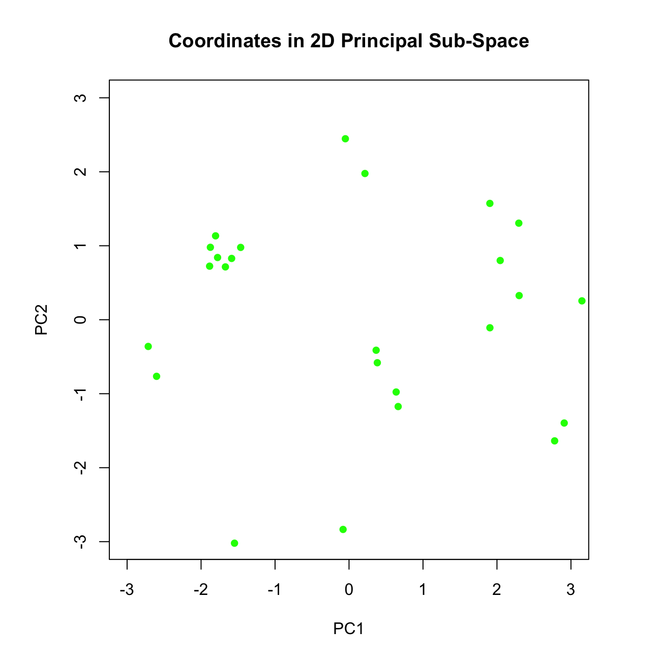

# The plot shows the coordinates (scores) obtained along the 1st and 2nd PC. 

# Create a new object which we will plot, such that this object contains x and 
# rotation variables oriented in the positive direction
pca_posDir <- pca 
pca_posDir$x <- scores
pca_posDir$rotation <- loadings

ggbiplot::ggbiplot(pca_posDir, labels = rownames(mtcars))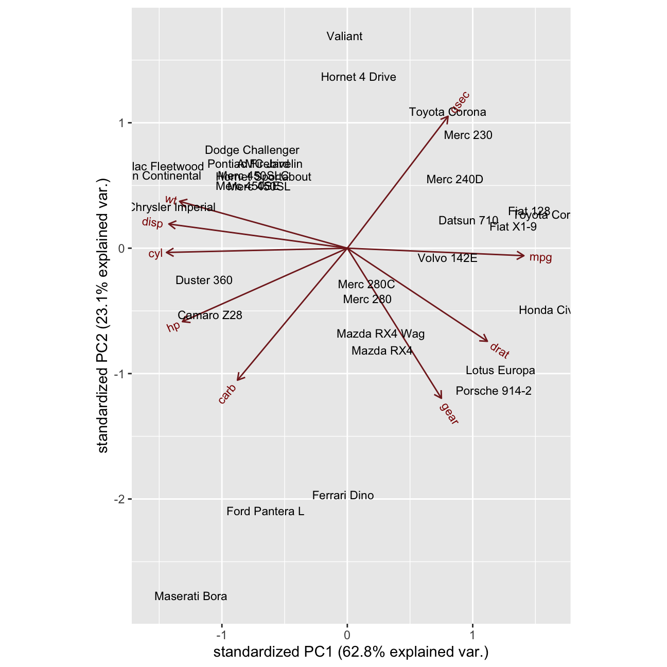

- When cars group together / are near each other in the biplot, what does it mean?

ANSWER: When cars group together, it indicates that they have similar features. In such a way we can identify our direct competitors in the market.

What can we say about the cars Ferrari, Ford Pantera L and Masserati?

ANSWER: These cars are quite similr to each other, mostly in terms of PC2. What is mostly similar about them is the fact that they are bascially very fast cars (what we can deduct from PC2 - [qsec + {-gear}]) Additionally, Maserati Bora is a high quality car with best features and effiency (PC1), where For Pantera L and Ferreri Dino tend to be also high quality cars, however not this efficient and featured.

Let’s improve the ggbiplot. I will do it using the ggbilot duntion, such that my labels are formed using row names, and the groups are formed using the countries provided. Also, I will alter the ggbiplot by removing the arrows from variable axes all together, such that the clusters are better revealed.

What can we say about the 3 potential clusters and their separation? ANSWER: Japanese and US cars are clearly different from each other, where European cars tends to be quite centrly located but also difer between each other a lot.
What are American cars characterised by?

ANSWER: American cars tend to have a good technology (right side of PC1) - strong engines (ho, disp, cyl), however they are quite heavy because of it. Therefore, they tend to have a tail in the group, that is not this fast (qsec). However, thanks to technology provided, they use less miles/ (US) gallon.

What are Japanese cars characterised by?

ANSWER: Japanese cars are not this petrol efficient, they use much more miles’(US) gallon (left side of PC1), however, they are much lighter. Thanks to it they tends to be in general a bit faster than American ones (more centered on PC2 than the oponents.

country <- c(rep("Japan", 3), rep("US",4), rep("Europe", 7),rep("US",3), "Europe", rep("Japan", 3), rep("US",4), rep("Europe", 3), "US", rep("Europe", 3))

#Biplot with variable axes
ggbiplot(pca, obs.scale = 1, var.scale = 1,
  groups = country, labels=rownames(mtcars) ,ellipse = TRUE, circle = TRUE) +
  scale_color_discrete(name = '') +
  theme(legend.direction = 'horizontal', legend.position = 'top')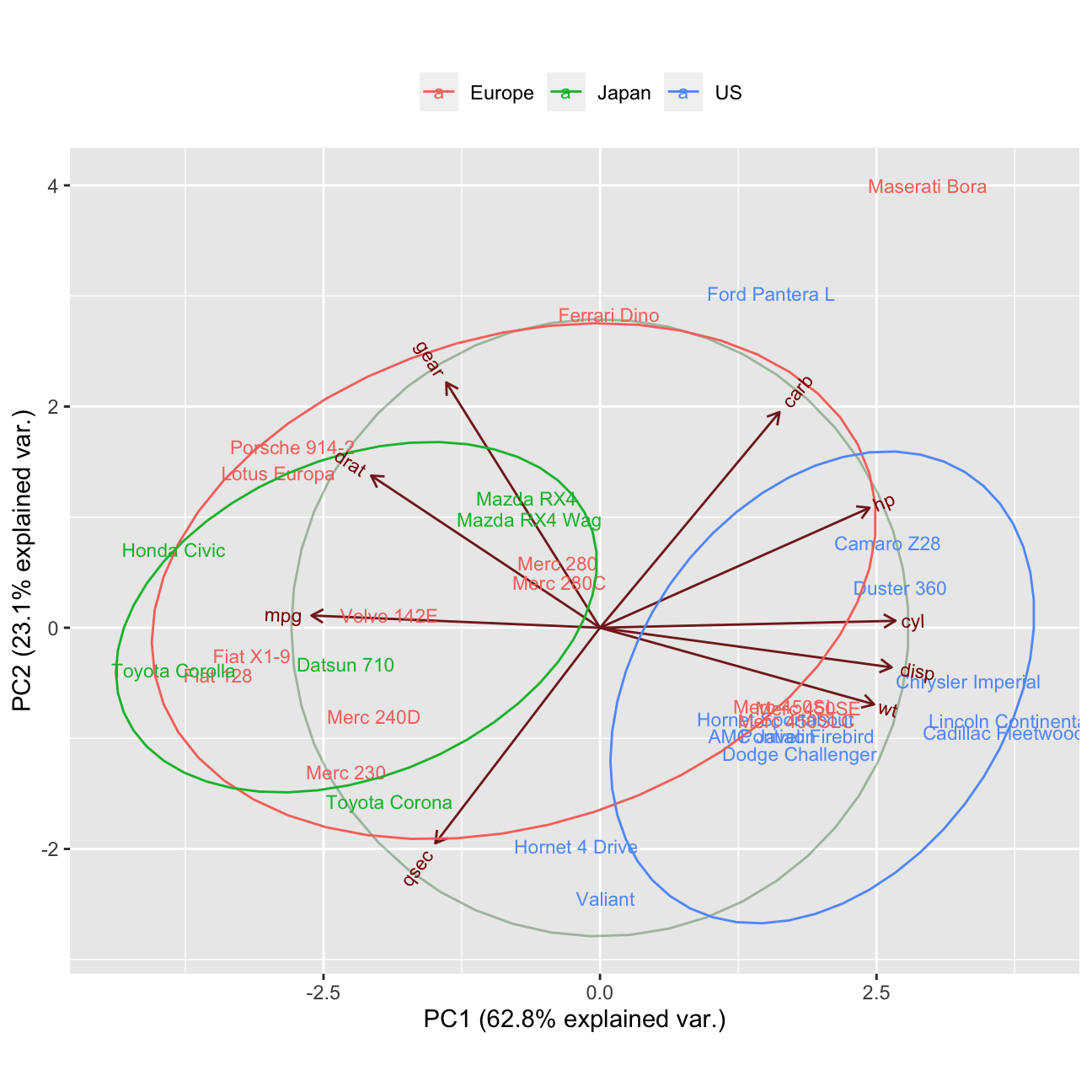

#Biplot without variable axes
ggbiplot(pca, obs.scale = 1, var.scale = 1,var.axes=FALSE,
  groups = country, labels=rownames(mtcars) ,ellipse = TRUE, circle = TRUE) +
  scale_color_discrete(name = '') +
  theme(legend.direction = 'horizontal', legend.position = 'top')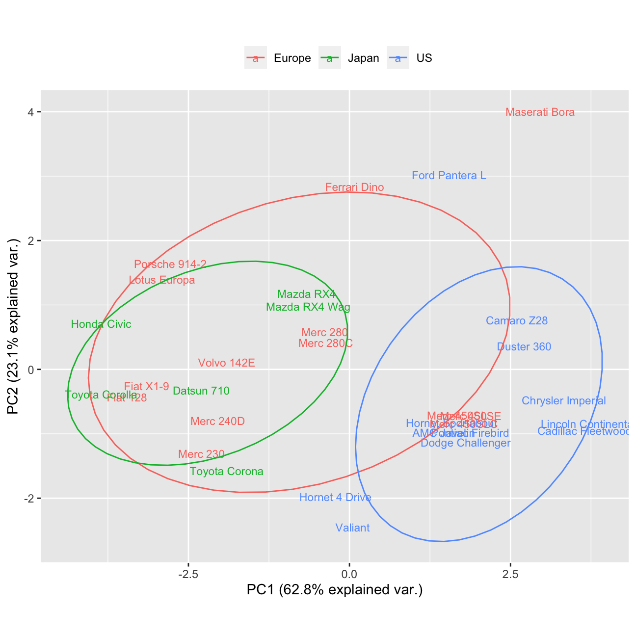

mtcars

##                      mpg cyl  disp  hp drat   wt qsec vs am gear carb
## Mazda RX4           21.0   6 160.0 110 3.90 2.62 16.5  0  1    4    4
## Mazda RX4 Wag       21.0   6 160.0 110 3.90 2.88 17.0  0  1    4    4
## Datsun 710          22.8   4 108.0  93 3.85 2.32 18.6  1  1    4    1
## Hornet 4 Drive      21.4   6 258.0 110 3.08 3.21 19.4  1  0    3    1
## Hornet Sportabout   18.7   8 360.0 175 3.15 3.44 17.0  0  0    3    2
## Valiant             18.1   6 225.0 105 2.76 3.46 20.2  1  0    3    1
## Duster 360          14.3   8 360.0 245 3.21 3.57 15.8  0  0    3    4
## Merc 240D           24.4   4 146.7  62 3.69 3.19 20.0  1  0    4    2
## Merc 230            22.8   4 140.8  95 3.92 3.15 22.9  1  0    4    2
## Merc 280            19.2   6 167.6 123 3.92 3.44 18.3  1  0    4    4
## Merc 280C           17.8   6 167.6 123 3.92 3.44 18.9  1  0    4    4
## Merc 450SE          16.4   8 275.8 180 3.07 4.07 17.4  0  0    3    3
## Merc 450SL          17.3   8 275.8 180 3.07 3.73 17.6  0  0    3    3
## Merc 450SLC         15.2   8 275.8 180 3.07 3.78 18.0  0  0    3    3
## Cadillac Fleetwood  10.4   8 472.0 205 2.93 5.25 18.0  0  0    3    4
## Lincoln Continental 10.4   8 460.0 215 3.00 5.42 17.8  0  0    3    4
## Chrysler Imperial   14.7   8 440.0 230 3.23 5.34 17.4  0  0    3    4
## Fiat 128            32.4   4  78.7  66 4.08 2.20 19.5  1  1    4    1
## Honda Civic         30.4   4  75.7  52 4.93 1.61 18.5  1  1    4    2
## Toyota Corolla      33.9   4  71.1  65 4.22 1.83 19.9  1  1    4    1
## Toyota Corona       21.5   4 120.1  97 3.70 2.46 20.0  1  0    3    1
## Dodge Challenger    15.5   8 318.0 150 2.76 3.52 16.9  0  0    3    2
## AMC Javelin         15.2   8 304.0 150 3.15 3.44 17.3  0  0    3    2
## Camaro Z28          13.3   8 350.0 245 3.73 3.84 15.4  0  0    3    4
## Pontiac Firebird    19.2   8 400.0 175 3.08 3.85 17.1  0  0    3    2
## Fiat X1-9           27.3   4  79.0  66 4.08 1.94 18.9  1  1    4    1
## Porsche 914-2       26.0   4 120.3  91 4.43 2.14 16.7  0  1    5    2
## Lotus Europa        30.4   4  95.1 113 3.77 1.51 16.9  1  1    5    2
## Ford Pantera L      15.8   8 351.0 264 4.22 3.17 14.5  0  1    5    4
## Ferrari Dino        19.7   6 145.0 175 3.62 2.77 15.5  0  1    5    6
## Maserati Bora       15.0   8 301.0 335 3.54 3.57 14.6  0  1    5    8
## Volvo 142E          21.4   4 121.0 109 4.11 2.78 18.6  1  1    4    2

Variance Analysis

I will perform variance analysis.

To recap: how many PCs do we have in total? ANSWER: We have 9 PCs in total.
I will check the amount of variance explained by each PC

# Proportion of Variance explained by each PC:
summary(pca)$importance

##                          PC1   PC2   PC3    PC4    PC5    PC6    PC7    PC8
## Standard deviation     2.378 1.443 0.710 0.5148 0.4280 0.3518 0.3241 0.2419
## Proportion of Variance 0.628 0.231 0.056 0.0295 0.0204 0.0138 0.0117 0.0065
## Cumulative Proportion  0.628 0.860 0.916 0.9453 0.9656 0.9794 0.9910 0.9975
##                            PC9
## Standard deviation     0.14896
## Proportion of Variance 0.00247
## Cumulative Proportion  1.00000

#                            PC1      PC2       PC3       PC4       PC5       PC6       PC7       PC8       PC9
#Standard deviation     2.378222 1.442948 0.7100809 0.5148082 0.4279704 0.3518426 0.3241326 0.2418962 0.1489644
#Proportion of Variance 0.628440 0.231340 0.0560200 0.0294500 0.0203500 0.0137500 0.0116700 0.0065000 0.0024700
#Cumulative Proportion  0.628440 0.859780 0.9158100 0.9452500 0.9656000 0.9793600 0.9910300 0.9975300 1.0000000

I obtain the total variance

X_scaled <- scale(mtcars, center = TRUE, scale = TRUE)
covX <- cov(X_scaled)
VT <- sum(diag(covX))
VT

## [1] 11

Summary: All the PCs except PC1 & PC2 show the standard deviation (variation) of less than 1. It means that there is no sense in using them as they explain less than 1 variable. In such a case we are better of using the original variable itself.

I will obtain the scree plot and establish where the ‘elbow’ occurs using fviz_screeplot() function such that labels showing percentages of variance explaiend are also shown on the plot.

fviz_screeplot(pca, addlabels = TRUE, ylim = c(0,100))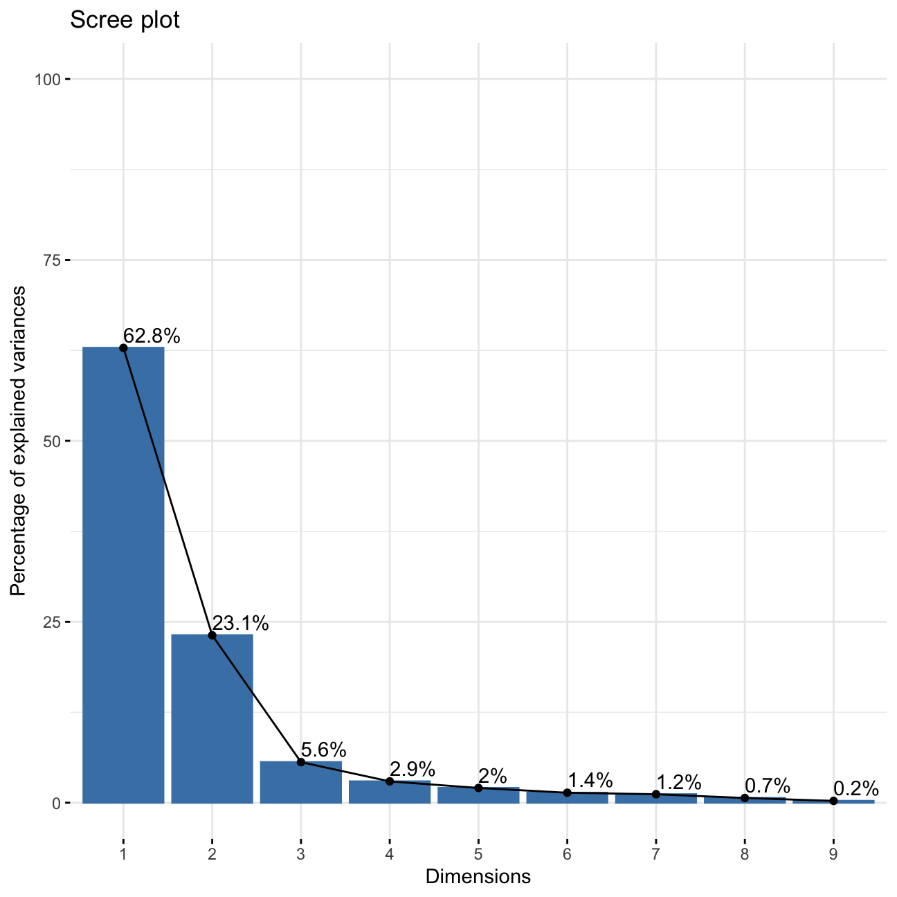

How many PCs should be kept?

ANSWER: We should use only PC1 and PC2 as they are the only ones that explain more than 10% of the data and whose variance is greater than 1.

PART 2: LINEAR DISCRIMINANT ANALYSIS

Theoretical Part

A definition of what is a discriminant.

ANSWER: A discriminant is a function that takes input vector $\mathbf{x}$ and assigns it to one and only one class $C_k$ out of $k$ classes.

What are the 2 assumptions for data such that LDA can be applied?

ANSWER: 1) The data should be composed of classes that are normally distributed and have equal covariances 2) No constant variables should be in the dataset.

Does data need to be normalised?

ANSWER: No, the data does not need to be neither centered nor scaled.

Is LDA a supervised or an unsupervised learning algorithm?

ANSWER: It is a supervised learning algorithm. It means that the LDA takes labels into account.

I will explain the effect the desired decision boundary should have on the projected data?

ANSWER: The decision boundary should be constructed in such a way that is easily assigns each point to one of the classes:

in case of 2 classes : the decision boundary is a line. It is defined by the equasion:

$𝑦(𝕩) = 𝕨^T𝕩 +w_0= 0$.

If the value of the point is >0, assign to class 1, otherwise, to class 2.

in case of K classes: Assign point 𝕩 to class:

$𝐶_k$ if $y_k(𝕩)>𝑦_j(𝕩)$

The decision boundary should not only not only separate well classes, but also maximise marigin between them.

What is the key performance criterion for LDA as opposed to PCA?

ANSWER: PCA aims to maximise variance, where LDA’s amin objective is to create groups (axes) that maximise class separation.

What is the ‘Difference of Class Means’ criterion of LDA? What is its limitation?

ANSWER: Maximise separation between projected class means:

$𝕨 ∝ (𝐦_2 −𝐦_1)$.

The problem with such an approach is that the points in to different classes may intermix and overlap.

the Fisher criterion.

ANSWER: States the same as “Difference of Class Means” criterion but at the same time it aims to minimize the variance of each class:

$𝕨 ∝ 𝕊_{W}^{-1}(𝐦_2 −𝐦_1)$.

Where

$𝕊_{W}$ is the Total within-class covariance matrix

Fisher cirterion’s goal is to also maximise the variance between classes. Such an appoach allows to create classes that are well separated.

Explain how minimisation of within class variance of each class helps with classification of the projected points?

ANSWER: As explained above, thanks to minimalisation of the variances within each class, we also maximise the variance between classes - it helps us to better separate the classes and prevent overlapping of data points and class intermixing. Such an apporach comes from differentiating the cost function

$J(\mathbb{w})$ to $𝕨 ∝ 𝕊_{W}^{-1}(𝐦_2 −𝐦_1)$.

Create Country Labels

I am going to continue working with the mtcars data set from above and utilise LDA for the classification purposes, such that I attempt to create K = 3 classes based on country of origin for each car.

The code below uses the variable you have created above, $\mathbb{X}$, stores the variable ${country}$ in the first column of $\mathbb{X}$ and calls that column ${label}$.

class(X) # X is a data frame

## [1] "data.frame"

country <- c(rep("Japan", 3), rep("US",4), rep("Europe", 7),rep("US",3), "Europe", 
             rep("Japan", 3), rep("US",4), rep("Europe", 3), "US", rep("Europe", 3))

X <- data.frame(cbind(label = country, X)) # (1 pt) data.frame; (1 pt) cbind

Pre-Process Data and Fit Model

I will now randomly shuffle the data, ensuring to keep the labels attached to correct observations. This will ensure that when I split the data into train/test sets next, I don’t by accident end up with all data of the same label in one set.

Then, I will fit LDA model to the training data set.

# randomly shuffle the data
set.seed(1234)
X_shuffled<- sample(nrow(X))
X_shuffled<- X[X_shuffled,]

# split into training / testing
set.seed(1234)
# Create the training dataset
train_test_split <- initial_split(X, prop = 0.75) #training set contains 75% of the data
set.seed(1234)
train_data <- training(train_test_split)
# Create the testing dataset
test_data <- testing(train_test_split)
# fit LDA using training data points
fit_LDA <- lda(formula= label ~ ., data = train_data) 

# print()
print(fit_LDA)

## Call:
## lda(label ~ ., data = train_data)
## 
## Prior probabilities of groups:
## Europe  Japan     US 
##  0.417  0.250  0.333 
## 
## Group means:
##         mpg  cyl disp    hp drat   wt qsec gear carb
## Europe 20.8 5.80  180 144.4 3.75 3.10 17.8 4.10 3.50
## Japan  25.1 4.67  116  87.8 4.08 2.29 18.4 3.83 2.17
## US     16.5 7.50  336 190.5 3.31 3.73 17.1 3.25 2.75
## 
## Coefficients of linear discriminants:
##          LD1     LD2
## mpg  -0.1366  0.0813
## cyl  -0.5826  0.6592
## disp  0.0464 -0.0272
## hp   -0.0152  0.0161
## drat -0.2672 -0.9257
## wt   -2.4450  3.5954
## qsec  0.3444 -0.2377
## gear  0.3703  1.9203
## carb  0.0208 -0.9191
## 
## Proportion of trace:
##   LD1   LD2 
## 0.831 0.169

I will now print out the fitted model and from the display, report what is the percentage of amount of between-group variance explained by each linear discriminant.

ANSWER: The amount of between-group variance explained by each LD is as follows: Proportion of trace: LD1 LD2 0.8308 0.1692 It can be understood as the pertentage of separation achieved by each discriminant function.

Is this a quantity that LDA aims to maximise?

ANSWER: Yes, this is indeed the number that LDA aims to maximise - the between-group variance.

Model Accuracy On Unseen Data

Next I will use the testing data set to investigate the accuracy of your model on unseen data (i.e. data not used during training).

Obtain predictions for train and test data sets.

#Predictions using stats library
predict_train <- predict(fit_LDA, newdata = train_data) # for the train dataset
predict_test <- predict(fit_LDA, newdata = test_data) # for the test dataset

I will produce 2 tables (one for each of the above) showing classification accuracy and explain the general meaning of values on the diagonal.

# Classification accuracy on training data
classTbl_train <- table(train_data$label, predict_train$class)
print(classTbl_train)

##         
##          Europe Japan US
##   Europe     10     0  0
##   Japan       2     4  0
##   US          0     0  8

# 2 errors occured - two actual Japanese cars predicted to belong to 'Europe' class

# Classification accuracy on testing data
classTbl_test <- table(test_data$label, predict_test$class)
print(classTbl_test)

##         
##          Europe Japan US
##   Europe      3     1  0
##   US          0     0  4

# 1 error occured - one actual European car predicted to belong to 'Japan' class

I obtain the same tables containing entries in a fraction format.

# Classification accuracy on training data in percent
prop.table(classTbl_train, 1)

##         
##          Europe Japan    US
##   Europe  1.000 0.000 0.000
##   Japan   0.333 0.667 0.000
##   US      0.000 0.000 1.000

# Classification accuracy on testing data in percent
prop_test<-prop.table(classTbl_test,1)
prop_test

##         
##          Europe Japan   US
##   Europe   0.75  0.25 0.00
##   US       0.00  0.00 1.00

I will now obtain and comment the total percent correct classification for training and testing data sets.

sum(diag(prop.table(classTbl_train))) #0.9166667

## [1] 0.917

#As for test set there are no predictions for the actual Japanese cars in seed 1234, I will count the acurracy manually
(prop_test[1,1]+prop_test[2,3])/2 #0.875

## [1] 0.875

Should we expect to obtain higher classification accuracy on a training or testing data?

ANSWER: I would expect the acurracy to be higher in the training set for two reasons - first of all, this is the data for which the model was trained. Second of all - the training data contains more rows than the testing data, so the mistake cost is automatically lower what we can see from the analysis above (2 errors in train_data, 1 error in test_data, however classification accuracy higher for training dataset. )