Building Recommendation Systems for BBC iPlayer users
Loading the Data
#Loadning the needed 2 datasets
movie_data <- fread(input="~/Documents/LBS/Machine Learning/Session 02/The Assignment/movies.csv",
                    stringsAsFactors = FALSE) #9742 number of rows

rating_data <- fread(input = "~/Documents/LBS/Machine Learning/Session 02/The Assignment/ratings.csv",nrows = 1e6) #100836 number of rows

#Creating the genre list for my data
list_genre <- c("Action", "Adventure", "Animation", "Children",
                "Comedy", "Crime","Documentary", "Drama", "Fantasy",
                "Film-Noir", "Horror", "Musical", "Mystery","Romance",
                "Sci-Fi", "Thriller", "War", "Western")
Cleaning the Data
Cleaning Movies Data
#Cleaning up the movie_data from the movies that appear more than once

#Finding the movies that appeard more than once
repeatMovies <- movie_data %>%
  group_by(title) %>%
  summarise(n = n()) %>%
  filter(n > 1) %>%
  pull(title)

repeatMovies # 5 movies appear more than once
## [1] "Confessions of a Dangerous Mind (2002)"
## [2] "Emma (1996)"
## [3] "Eros (2004)"
## [4] "Saturn 3 (1980)"
## [5] "War of the Worlds (2005)"# [1] "Confessions of a Dangerous Mind (2002)" "Emma (1996)"
# [3] "Eros (2004)" "Saturn 3 (1980)"
# [5] "War of the Worlds (2005)"
removeRows <- 0 #Initialising the variable that stores the rows we have to remove later (the duplicates)
##### REMOVE REPEATS IN RATING DATA ####
for(i in repeatMovies){
repeatMovieLoc <- which(movie_data$title == i) #Getting the indices of the rows where the current movie (with title i) is stored
tempGenre <- paste(movie_data$genres[repeatMovieLoc], collapse="|") #Collapsing the genres assigned to the duplicated movies, separated by |
tempGenre <- paste(unique(unlist(strsplit(tempGenre, split = "\\|")[[1]])), collapse = "|") #Splitting the string up again, taking only the unique values
movie_data$genres[repeatMovieLoc[1]] <- tempGenre #Bringing the new genre string to the first appearance of the movie in the dataframe
removeRows <- c(removeRows, repeatMovieLoc[-1]) #Adding the duplicate entry (row 6271) to the list of rows I want to remove later
### REMOVE DUPLICATES IN RATINGS DATA ###
repeatMovieIdLoc <- which(rating_data$movieId %in% movie_data$movieId[removeRows]) #Searching for all the entries in the rating_data dataframe that refer to duplicate movies in movie_data
rating_data$movieId[repeatMovieIdLoc] <- movie_data$movieId[repeatMovieLoc[1]] #Changing movieId to the movieId that remains in our movie_data dataframe
}
#Removing the duplicate rows in the movie_data
movie_data <- movie_data[-removeRows,]
movie_data## movieId title
## 1: 1 Toy Story (1995)
## 2: 2 Jumanji (1995)
## 3: 3 Grumpier Old Men (1995)
## 4: 4 Waiting to Exhale (1995)
## 5: 5 Father of the Bride Part II (1995)
## ---
## 9733: 193581 Black Butler: Book of the Atlantic (2017)
## 9734: 193583 No Game No Life: Zero (2017)
## 9735: 193585 Flint (2017)
## 9736: 193587 Bungo Stray Dogs: Dead Apple (2018)
## 9737: 193609 Andrew Dice Clay: Dice Rules (1991)
## genres
## 1: Adventure|Animation|Children|Comedy|Fantasy
## 2: Adventure|Children|Fantasy
## 3: Comedy|Romance
## 4: Comedy|Drama|Romance
## 5: Comedy
## ---
## 9733: Action|Animation|Comedy|Fantasy
## 9734: Animation|Comedy|Fantasy
## 9735: Drama
## 9736: Action|Animation
## 9737: ComedyCleaning Ratings Data
There is a risk that the same user has rated a movie multiple times. I would like to keep only the best rating.
I will group by userId and movieId, and only take the highest (maximum) rating In the end, I will produce a dataframe, where there is (at most) 1 rating of a user for a movie. This is a constraint needed to build up a proper user-movie-interaction-matrix
rating_data <- rating_data %>%
  group_by(userId, movieId) %>%
  summarise(rating = max(rating)) %>%
  ungroup()

length(unique(rating_data$movieId)) #Identifying movies that have not been yet rated by any user. They are safe to ignore for now, since they shouldn't affect our recommendations
## [1] 9719length(unique(movie_data$movieId))## [1] 9737setdiff(unique(movie_data$movieId), unique(rating_data$movieId)) ## [1] 1076 2939 3338 3456 4194 5721 6668 6849 7020 7792 8765 25855
## [13] 26085 30892 32160 32371 34482 85565rating_data## # A tibble: 100,832 x 3
## userId movieId rating
## <int> <int> <dbl>
## 1 1 1 4
## 2 1 3 4
## 3 1 6 4
## 4 1 47 5
## 5 1 50 5
## 6 1 70 3
## 7 1 101 5
## 8 1 110 4
## 9 1 151 5
## 10 1 157 5
## # … with 100,822 more rowsChecking the Data is Clean
#movie_data
skim(movie_data)| Name | movie_data |
| Number of rows | 9737 |
| Number of columns | 3 |
| _______________________ | |
| Column type frequency: | |
| character | 2 |
| numeric | 1 |
| ________________________ | |
| Group variables | None |
Variable type: character
| skim_variable | n_missing | complete_rate | min | max | empty | n_unique | whitespace |
|---|---|---|---|---|---|---|---|
| title | 0 | 1 | 6 | 158 | 0 | 9737 | 0 |
| genres | 0 | 1 | 3 | 77 | 0 | 952 | 0 |
Variable type: numeric
| skim_variable | n_missing | complete_rate | mean | sd | p0 | p25 | p50 | p75 | p100 | hist |
|---|---|---|---|---|---|---|---|---|---|---|
| movieId | 0 | 1 | 42165 | 52136 | 1 | 3247 | 7294 | 76173 | 193609 | ▇▂▂▁▁ |
summary(movie_data) ## movieId title genres
## Min. : 1 Length:9737 Length:9737
## 1st Qu.: 3247 Class :character Class :character
## Median : 7294 Mode :character Mode :character
## Mean : 42165
## 3rd Qu.: 76173
## Max. :193609head(movie_data)## movieId title
## 1: 1 Toy Story (1995)
## 2: 2 Jumanji (1995)
## 3: 3 Grumpier Old Men (1995)
## 4: 4 Waiting to Exhale (1995)
## 5: 5 Father of the Bride Part II (1995)
## 6: 6 Heat (1995)
## genres
## 1: Adventure|Animation|Children|Comedy|Fantasy
## 2: Adventure|Children|Fantasy
## 3: Comedy|Romance
## 4: Comedy|Drama|Romance
## 5: Comedy
## 6: Action|Crime|Thriller#rating_data
skim(movie_data)| Name | movie_data |
| Number of rows | 9737 |
| Number of columns | 3 |
| _______________________ | |
| Column type frequency: | |
| character | 2 |
| numeric | 1 |
| ________________________ | |
| Group variables | None |
Variable type: character
| skim_variable | n_missing | complete_rate | min | max | empty | n_unique | whitespace |
|---|---|---|---|---|---|---|---|
| title | 0 | 1 | 6 | 158 | 0 | 9737 | 0 |
| genres | 0 | 1 | 3 | 77 | 0 | 952 | 0 |
Variable type: numeric
| skim_variable | n_missing | complete_rate | mean | sd | p0 | p25 | p50 | p75 | p100 | hist |
|---|---|---|---|---|---|---|---|---|---|---|
| movieId | 0 | 1 | 42165 | 52136 | 1 | 3247 | 7294 | 76173 | 193609 | ▇▂▂▁▁ |
summary(rating_data) ## userId movieId rating
## Min. : 1 Min. : 1 Min. :0.5
## 1st Qu.:177 1st Qu.: 1199 1st Qu.:3.0
## Median :325 Median : 2991 Median :3.5
## Mean :326 Mean : 19430 Mean :3.5
## 3rd Qu.:477 3rd Qu.: 8119 3rd Qu.:4.0
## Max. :610 Max. :193609 Max. :5.0head(rating_data)## # A tibble: 6 x 3
## userId movieId rating
## <int> <int> <dbl>
## 1 1 1 4
## 2 1 3 4
## 3 1 6 4
## 4 1 47 5
## 5 1 50 5
## 6 1 70 3dupes_movie<-movie_data%>%get_dupes(movieId,title) # checking for dupes once again
dupes_movie # no dupes## Empty data.table (0 rows and 4 cols): movieId,title,dupe_count,genresdupes_rating<-rating_data%>%get_dupes(userId,movieId)
dupes_rating # no dupes## # A tibble: 0 x 4
## # … with 4 variables: userId <int>, movieId <int>, dupe_count <int>,
## # rating <dbl>movie_data## movieId title
## 1: 1 Toy Story (1995)
## 2: 2 Jumanji (1995)
## 3: 3 Grumpier Old Men (1995)
## 4: 4 Waiting to Exhale (1995)
## 5: 5 Father of the Bride Part II (1995)
## ---
## 9733: 193581 Black Butler: Book of the Atlantic (2017)
## 9734: 193583 No Game No Life: Zero (2017)
## 9735: 193585 Flint (2017)
## 9736: 193587 Bungo Stray Dogs: Dead Apple (2018)
## 9737: 193609 Andrew Dice Clay: Dice Rules (1991)
## genres
## 1: Adventure|Animation|Children|Comedy|Fantasy
## 2: Adventure|Children|Fantasy
## 3: Comedy|Romance
## 4: Comedy|Drama|Romance
## 5: Comedy
## ---
## 9733: Action|Animation|Comedy|Fantasy
## 9734: Animation|Comedy|Fantasy
## 9735: Drama
## 9736: Action|Animation
## 9737: ComedysearchMatrix <- movie_data %>%
separate_rows(genres, sep = "\\|") %>% #Splitting the genres assigned to movies into multiple rows
mutate(values = 1) %>%
pivot_wider(names_from = genres, values_from = values) %>% #Pivoting the dataframe so that each genre is assigned its own column
replace(is.na(.), 0)
searchMatrix %>% #Some movies have no genres listed, this is not problematic for the recommendation model, since it is purely collaborative, rather than content-based
filter(`(no genres listed)`==1) %>%
length()## [1] 22Building the Rating Matrix (User-Movie-Interactions Matrix)
ratingMatrix <- rating_data %>% #A ratings matrix consists of userId's as rows and movieId's as columns
  arrange(movieId) %>%
  pivot_wider(names_from = movieId, values_from = rating) %>%   #allocating each movie to its own column
  arrange(userId) %>%
  select(-userId)   #dropping userId


ratingMatrix <- as.matrix(ratingMatrix) #converting the dataframe created above into a matrix

#Ordering the rows and columns so that those with the fewest NAs are furthest to the top left, which is crucial for selecting the most popular movies and most frequent users
ratingMatrix <- ratingMatrix[order(rowSums(is.na(ratingMatrix))),order(colSums(is.na(ratingMatrix)))]


ratingMatrix <- as(ratingMatrix, "realRatingMatrix") #Converting the rating matrix into a recommenderlab sparse matrix
STEP 1 - EXPLORATORY ANALYSIS
Preparing the Data
Ratings Counts
rating_data %>%
  group_by(rating) %>%
  summarise(n = n()) #Creating a count of movie ratings
## # A tibble: 10 x 2
## rating n
## <dbl> <int>
## 1 0.5 1370
## 2 1 2811
## 3 1.5 1791
## 4 2 7550
## 5 2.5 5550
## 6 3 20047
## 7 3.5 13134
## 8 4 26817
## 9 4.5 8551
## 10 5 13211movie_rating_count <- rating_data %>%
group_by(movieId) %>%
summarise(ratings = n()) %>%
left_join(movie_data, by = "movieId") %>%
select(movieId, title, ratings) %>%
arrange(desc(ratings)) #Creating a table with number of ratings per movie
head(movie_rating_count) #previewing ## # A tibble: 6 x 3
## movieId title ratings
## <int> <chr> <int>
## 1 356 Forrest Gump (1994) 329
## 2 318 Shawshank Redemption, The (1994) 317
## 3 296 Pulp Fiction (1994) 307
## 4 593 Silence of the Lambs, The (1991) 279
## 5 2571 Matrix, The (1999) 278
## 6 260 Star Wars: Episode IV - A New Hope (1977) 251user_rating_count <- rating_data %>% #Creating a table with number of ratings per user
group_by(userId) %>%
summarise(ratings = n()) %>%
arrange(desc(ratings))
head(user_rating_count) #preaviewing## # A tibble: 6 x 2
## userId ratings
## <int> <int>
## 1 414 2698
## 2 599 2478
## 3 474 2108
## 4 448 1864
## 5 274 1346
## 6 610 1302How similar the 100 most popular movies are to eachother
movie_similarity <- similarity(ratingMatrix[, 1:100],
                               method = "cosine",
                               which = "items")


movie_similarity <- as.matrix(movie_similarity) + diag(100) #Adding diag(100) - the similarity of a movie with itself is always 1

image(movie_similarity, main = "Top 100 Popular Movies' Similarity")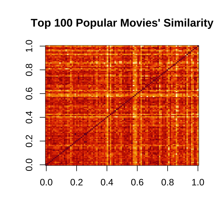
How similar the 100 most frequent users are to eachother
#I produce a matrix which calculates how similar users are to one another
user_similarity <- similarity(ratingMatrix[1:100, ],
                              method = "cosine",
                              which = "users")

#I also add diag(100), since the similarity of a user with themselves is 1
user_similarity <- as.matrix(user_similarity) + diag(100)

image(user_similarity, main = "100 Top active users' similarity")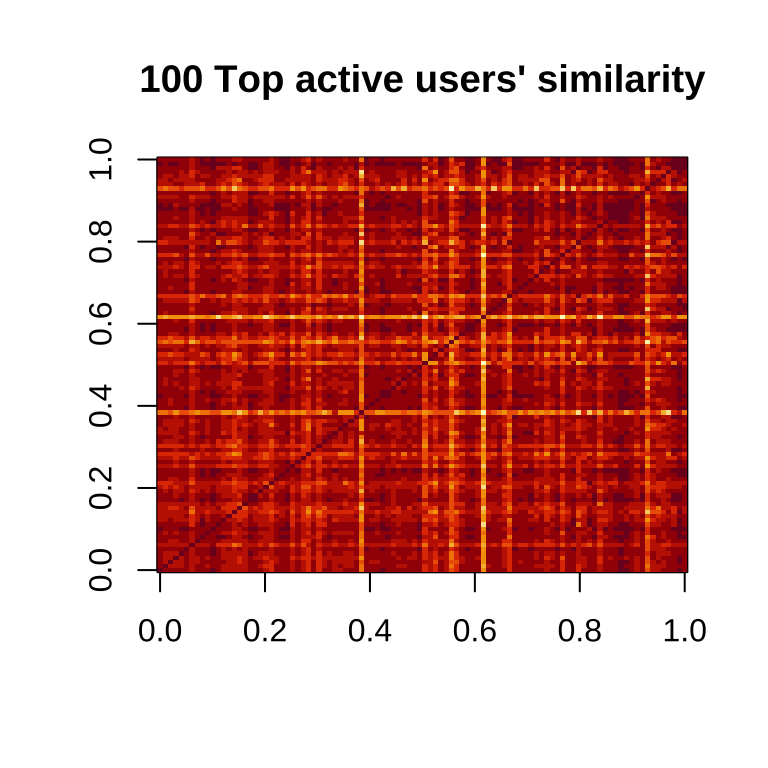
a Histogram Showing the Frequency of Ratings of All Movies
rating_data %>%
  group_by(rating) %>%
  count()
## # A tibble: 10 x 2
## # Groups: rating [10]
## rating n
## <dbl> <int>
## 1 0.5 1370
## 2 1 2811
## 3 1.5 1791
## 4 2 7550
## 5 2.5 5550
## 6 3 20047
## 7 3.5 13134
## 8 4 26817
## 9 4.5 8551
## 10 5 13211rating_data %>% #Building a histogram
ggplot(aes(rating)) +
geom_bar() +
labs(title="Movies were most frequently rated for 4.0 ",subtitle = "Movie rating frequency",x="Rating",y="Count") +
theme_minimal() +
theme(plot.title = element_text(color = "gray60",size=15,face="bold", family= "Montserrat"),
axis.title.y = element_text(size = 8, angle = 90, family="Montserrat", face = "plain"),
plot.subtitle = element_text(color = "gray60", face="plain", ,size= 10,family= "Montserrat"),
axis.title.x = element_text(size = 8, family="Montserrat", face = "plain"),
axis.text.x=element_text(family="Montserrat", size=7),
axis.text.y=element_text(family="Montserrat", size=7))+
scale_x_continuous(limits=c(0,5.5)) +
scale_y_continuous(limits=c(0,30000))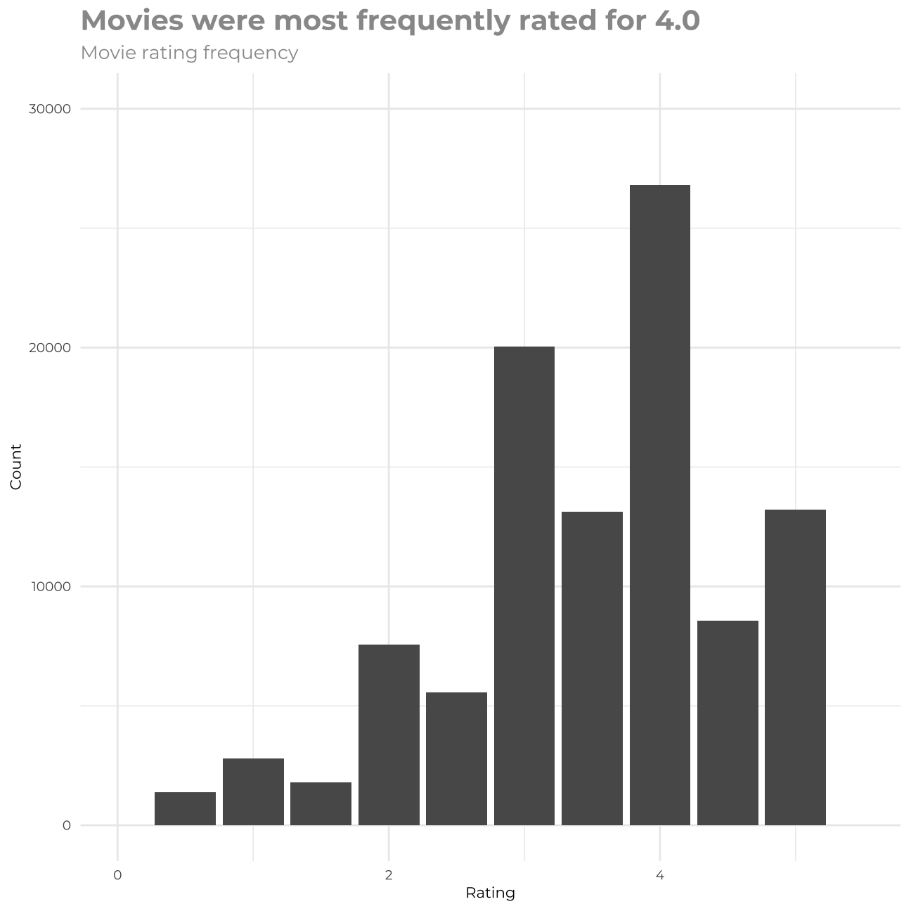
(rating_data)## # A tibble: 100,832 x 3
## userId movieId rating
## <int> <int> <dbl>
## 1 1 1 4
## 2 1 3 4
## 3 1 6 4
## 4 1 47 5
## 5 1 50 5
## 6 1 70 3
## 7 1 101 5
## 8 1 110 4
## 9 1 151 5
## 10 1 157 5
## # … with 100,822 more rowsSTEP 2 - SELECT MOST COMMON USERS AND MOVIES
I will select movies with more than ‘m’ ratings and users who have given more than ‘n’ ratings, where m <- c(10, 20, 50, 100, 200); n <- m
#Since the rows (users) and columns (movies) of my ratingMatrix are already ranked in decreasing order of frequency/popularity, we are just slicing the matrix

#movies rated more than 10 times and users who have rated more than 10 movies
top10_rate <- ratingMatrix[rowCounts(ratingMatrix) > 10,colCounts(ratingMatrix) > 10]

#movies rated more than 20 times and users who have rated more than 20 movies
top20_rate <- ratingMatrix[rowCounts(ratingMatrix) > 20,colCounts(ratingMatrix) > 20]

#movies rated more than 50 times and users who have rated more than 50 movies
top50_rate <- ratingMatrix[rowCounts(ratingMatrix) > 50,colCounts(ratingMatrix) > 50]

#movies rated more than 100 times and users who have rated more than 100 movies
top100_rate <- ratingMatrix[rowCounts(ratingMatrix) > 100,colCounts(ratingMatrix) > 100]
#top100_rate <- top100_rate[rowCounts(top100_rate) > 5, ]

#movies rated more than 200 times and users who have rated more than 200 movies
top200_rate <- ratingMatrix[rowCounts(ratingMatrix) > 200,colCounts(ratingMatrix) > 200]
STEP 3 - BUILDING RECOMMENDATION SYSTEMS
For building and testing my recommendation systems I built matrixes with movies containing more than m ratings and users who rated more than n movies, where n=m. I selected the following values of m & n to test: 10,20,50,100, 200. For each of the values I ran three models using methods: - User-user memory-based method (UBCF) - Item-item memory-based method (IBCF) Both of the above are memory based, collaborative filtering methods that learn from the past interactions between users/items to make new recommendations. The assumption behind these is that we have a sufficient number of interaction data in order for our predictions to a) establish similarities between users/items b) predict reliable outcomes. - Model-based approach using matrix factorisation (LIMBF) This method is based on user-item interactions, it allows for a level of approximation for groups or individuals, we can establish a mathematical level of confidence on the model. The drawback of this approach is that it works much slower and demands much bigger computing power to execute – it is much more costly to run.
Splitting each subset into test and training data
set.seed(1234) # setting seed
top10_split <- evaluationScheme(top10_rate, method="split", train=0.8, given=-5) # splitting all the data to 80% training data and 20% remaining for the testing
top10_split
## Evaluation scheme using all-but-5 items
## Method: 'split' with 1 run(s).
## Training set proportion: 0.800
## Good ratings: NA
## Data set: 610 x 2121 rating matrix of class 'realRatingMatrix' with 79636 ratings.set.seed(1234)
top20_rate <- top20_rate[rowCounts(top20_rate) > 5, ]
top20_split <- evaluationScheme(top20_rate, method="split", train=0.8, given=-5)
top20_split## Evaluation scheme using all-but-5 items
## Method: 'split' with 1 run(s).
## Training set proportion: 0.800
## Good ratings: NA
## Data set: 595 x 1235 rating matrix of class 'realRatingMatrix' with 66401 ratings.set.seed(1234)
top50_split <- evaluationScheme(top50_rate, method="split", train=0.8, given=-5)
top50_split## Evaluation scheme using all-but-5 items
## Method: 'split' with 1 run(s).
## Training set proportion: 0.800
## Good ratings: NA
## Data set: 378 x 436 rating matrix of class 'realRatingMatrix' with 36214 ratings.set.seed(1234)
top100_rate <- top100_rate[rowCounts(top100_rate) > 5, ]
top100_split <- evaluationScheme(top100_rate, method="split", train=0.8, given=-5)
set.seed(1234)
top200_rate <- top200_rate[rowCounts(top200_rate) > 5, ]
top200_split <- evaluationScheme(top200_rate, method="split", train=0.8, given=-5)I will build three separate recommendations systems for each of the values of ‘n’ and ‘m’ (5 versions for each type of RS)
Item Based CF
#TOP10
set.seed(1234) # setting seed
top10_IBCF <- Recommender(getData(top10_split, "train"), method = "IBCF", param=list(normalize = "center", method="Cosine",k=350))
#TOP20
set.seed(1234) # setting seed
top20_IBCF <- Recommender(getData(top20_split, "train"), method = "IBCF", param=list(normalize = "center", method="Cosine",k=350))
#TOP50
set.seed(1234) # setting seed
top50_IBCF <- Recommender(getData(top50_split, "train"), method = "IBCF", param=list(normalize = "center", method="Cosine",k=350))
#TOP100
set.seed(1234) # setting seed
top100_IBCF <- Recommender(getData(top100_split, "train"), method = "IBCF", param=list(normalize = "center", method="Cosine",k=350))
#TOP200
set.seed(1234) # setting seed
top200_IBCF <- Recommender(getData(top200_split, "train"), method = "IBCF", param=list(normalize = "center", method="Cosine",k=350))
User Based CF
#TOP10
set.seed(1234) # setting seed
top10_UBCF <- Recommender(getData(top10_split, "train"), method = "UBCF", param=list(normalize = "center", method="Cosine", nn=25))
#TOP20
set.seed(1234) # setting seed
top20_UBCF <- Recommender(getData(top20_split, "train"), method = "UBCF", param=list(normalize = "center", method="Cosine", nn=25))
#TOP50
set.seed(1234) # setting seed
top50_UBCF <- Recommender(getData(top50_split, "train"), method = "UBCF", param=list(normalize = "center", method="Cosine", nn=25))
#TOP100
set.seed(1234) # setting seed
top100_UBCF <- Recommender(getData(top100_split, "train"), method = "UBCF", param=list(normalize = "center", method="Cosine", nn=25))
#TOP200
set.seed(1234) # setting seed
top200_UBCF <- Recommender(getData(top200_split, "train"), method = "UBCF", param=list(normalize = "center", method="Cosine", nn=25))
Model Based CF using Matrix Factorisation
#TOP10
set.seed(1234) # setting seed
top10_LIBMF <- Recommender(getData(top10_split, "train"), method = "LIBMF", param=list(normalize = "center", method="Cosine"))
## Available parameter (with default values):
## dim = 10
## costp_l2 = 0.01
## costq_l2 = 0.01
## nthread = 1
## verbose = FALSE#TOP20
set.seed(1234) # setting seed
top20_LIBMF <- Recommender(getData(top20_split, "train"), method = "LIBMF", param=list(normalize = "center", method="Cosine"))## Available parameter (with default values):
## dim = 10
## costp_l2 = 0.01
## costq_l2 = 0.01
## nthread = 1
## verbose = FALSE#TOP50
set.seed(1234) # setting seed
top50_LIBMF <- Recommender(getData(top50_split, "train"), method = "LIBMF", param=list(normalize = "center", method="Cosine"))## Available parameter (with default values):
## dim = 10
## costp_l2 = 0.01
## costq_l2 = 0.01
## nthread = 1
## verbose = FALSE#TOP100
set.seed(1234) # setting seed
top100_LIBMF <- Recommender(getData(top100_split, "train"), method = "LIBMF", param=list(normalize = "center", method="Cosine"))## Available parameter (with default values):
## dim = 10
## costp_l2 = 0.01
## costq_l2 = 0.01
## nthread = 1
## verbose = FALSE#TOP200
set.seed(1234) # setting seed
top200_LIBMF <- Recommender(getData(top200_split, "train"), method = "LIBMF", param=list(normalize = "center", method="Cosine"))## Available parameter (with default values):
## dim = 10
## costp_l2 = 0.01
## costq_l2 = 0.01
## nthread = 1
## verbose = FALSEIn my work, I built in total 15 models. However, before I did it, I set the seed for ‘1234’ in order to split the data for each mxn matrix. It is important to mention, as one of the remarks from the analysis I realized is that the outcome and performance of the models is strongly dependent on the seed we choose. Using different seeds at the end led me to the same model choice, however, the outputs differed significantly from each other. Let me now explain how the models behave when we include only common movies/users first. When n and m= 200, we include in our model only the movies that were rated 200 or more times and the users that rated more than 200 movies. In such a manner, we significantly shrink the data. As a result, even though the RMSE is low in comparison to other models, our dataset does not have many values and it is not fully reliable. On the contrary, when we set our n and m=10 or 20, we include also rarely watched movies and not so active users. In this way, we obtain a large dataset including the majority of the observations. However, if we include such rare items/ users, our models have much less predictive power, and that ultimately lead us to higher RMSE. As we will see further from the RMSE analysis, the best choice lies in between, when n & m =100 or 50. The middle point seems to be the tradeoff of the two options mentioned above.
STEP 4 - Computing RMSE of each model and combination of m x n
I will assess performance of the above models for different number of ‘items’ and ‘users’. I need to remember CF methods are most appropriate for high volume items (often watched movies) and frequent users. So, if I use n,m == 20 then performance changes as opposed to when I use n, == 50.
For each recommendation system we expect to see 5 RMSE numbers, corresponding to n,m == {10,20,50,100,200}
RMSE_item_based_CF
set.seed(1234) # setting seed
#TOP10

#I compute predicted ratings by giving the model the known part of the test data (i.e. the data of the users for all but 5 movies for each user)
set.seed(1234) # setting seed
top10_IBCF_predict <- predict(top10_IBCF, getData(top10_split, "known"), type="ratings")

#Finally, I can calculate RMSE between the predictions and the unknown part of the test data (i.e. for the 5 movies that were held out)
set.seed(1234) # setting seed
top10_IBCF_RMSE <- calcPredictionAccuracy(top10_IBCF_predict, getData(top10_split, "unknown"))[1]
top10_IBCF_RMSE
## RMSE
## 1.12#TOP20
#I compute predicted ratings by giving the model the known part of the test data (i.e. the data of the users for all but 5 movies for each user)
set.seed(1234) # setting seed
top20_IBCF_predict <- predict(top20_IBCF, getData(top20_split, "known"), type="ratings")
#Finally, I can calculate RMSE between the predictions and the unknown part of the test data (i.e. for the 5 movies that were held out)
set.seed(1234) # setting seed
top20_IBCF_RMSE <- calcPredictionAccuracy(top20_IBCF_predict, getData(top20_split, "unknown"))[1]
top20_IBCF_RMSE## RMSE
## 1.05#TOP20
#I compute predicted ratings by giving the model the known part of the test data (i.e. the data of the users for all but 5 movies for each user)
set.seed(1234) # setting seed
top50_IBCF_predict <- predict(top50_IBCF, getData(top50_split, "known"), type="ratings")
#Finally, I can calculate RMSE between the predictions and the unknown part of the test data (i.e. for the 5 movies that were held out)
set.seed(1234) # setting seed
top50_IBCF_RMSE <- calcPredictionAccuracy(top50_IBCF_predict, getData(top50_split, "unknown"))[1]
top50_IBCF_RMSE## RMSE
## 0.848#TOP20
#I compute predicted ratings by giving the model the known part of the test data (i.e. the data of the users for all but 5 movies for each user)
set.seed(1234) # setting seed
top100_IBCF_predict <- predict(top100_IBCF, getData(top100_split, "known"), type="ratings")
#Finally, I can calculate RMSE between the predictions and the unknown part of the test data (i.e. for the 5 movies that were held out)
set.seed(1234) # setting seed
top100_IBCF_RMSE <- calcPredictionAccuracy(top100_IBCF_predict, getData(top100_split, "unknown"))[1]
top100_IBCF_RMSE## RMSE
## 0.823#TOP200
#I compute predicted ratings by giving the model the known part of the test data (i.e. the data of the users for all but 5 movies for each user)
set.seed(1234) # setting seed
top200_IBCF_predict <- predict(top200_IBCF, getData(top200_split, "known"), type="ratings")
#Finally, I can calculate RMSE between the predictions and the unknown part of the test data (i.e. for the 5 movies that were held out)
set.seed(1234) # setting seed
top200_IBCF_RMSE <- calcPredictionAccuracy(top200_IBCF_predict, getData(top200_split, "unknown"))[1]
top200_IBCF_RMSE## RMSE
## 0.815RMSE_user_based_CF
set.seed(1234) # setting seed
#TOP10
top10_UBCF_predict <- predict(top10_UBCF, getData(top10_split, "known"), type="ratings")

set.seed(1234) # setting seed
top10_UBCF_RMSE <- calcPredictionAccuracy(top10_UBCF_predict, getData(top10_split, "unknown"))[1]
top10_UBCF_RMSE
## RMSE
## 1.15#TOP20
set.seed(1234) # setting seed
top20_UBCF_predict <- predict(top20_UBCF, getData(top20_split, "known"), type="ratings")
set.seed(1234) # setting seed
top20_UBCF_RMSE <- calcPredictionAccuracy(top20_UBCF_predict, getData(top20_split, "unknown"))[1]
top20_UBCF_RMSE## RMSE
## 1.24#TOP50
set.seed(1234) # setting seed
top50_UBCF_predict <- predict(top50_UBCF, getData(top50_split, "known"), type="ratings")
set.seed(1234) # setting seed
top50_UBCF_RMSE <- calcPredictionAccuracy(top50_UBCF_predict, getData(top50_split, "unknown"))[1]
top50_UBCF_RMSE## RMSE
## 0.975#TOP100
set.seed(1234) # setting seed
top100_UBCF_predict <- predict(top100_UBCF, getData(top100_split, "known"), type="ratings")
set.seed(1234) # setting seed
top100_UBCF_RMSE <- calcPredictionAccuracy(top100_UBCF_predict, getData(top100_split, "unknown"))[1]
top100_UBCF_RMSE## RMSE
## 0.868#TOP200
set.seed(1234) # setting seed
top200_UBCF_predict <- predict(top200_UBCF, getData(top200_split, "known"), type="ratings")
set.seed(1234) # setting seed
top200_UBCF_RMSE <- calcPredictionAccuracy(top200_UBCF_predict, getData(top200_split, "unknown"))[1]
top200_UBCF_RMSE## RMSE
## 0.827RMSE_model_based_CF_using_MF
set.seed(1234) # setting seed
#TOP10
top10_LIBMF_predict <- predict(top10_LIBMF, getData(top10_split, "known"), type="ratings")
## iter tr_rmse obj
## 0 1.1798 1.1613e+05
## 1 0.8518 6.3520e+04
## 2 0.8295 6.0723e+04
## 3 0.8056 5.7777e+04
## 4 0.7878 5.5632e+04
## 5 0.7759 5.4206e+04
## 6 0.7670 5.3179e+04
## 7 0.7604 5.2403e+04
## 8 0.7547 5.1748e+04
## 9 0.7497 5.1182e+04
## 10 0.7453 5.0694e+04
## 11 0.7411 5.0221e+04
## 12 0.7373 4.9807e+04
## 13 0.7335 4.9405e+04
## 14 0.7298 4.8997e+04
## 15 0.7261 4.8591e+04
## 16 0.7227 4.8231e+04
## 17 0.7192 4.7871e+04
## 18 0.7158 4.7514e+04
## 19 0.7124 4.7146e+04set.seed(1234) # setting seed
top10_LIBMF_RMSE <- calcPredictionAccuracy(top10_LIBMF_predict, getData(top10_split, "unknown"))[1]
top10_LIBMF_RMSE## RMSE
## 0.874#TOP20
set.seed(1234) # setting seed
top20_LIBMF_predict <- predict(top20_LIBMF, getData(top20_split, "known"), type="ratings")## iter tr_rmse obj
## 0 1.1637 9.4129e+04
## 1 0.8500 5.2580e+04
## 2 0.8308 5.0597e+04
## 3 0.8094 4.8412e+04
## 4 0.7938 4.6822e+04
## 5 0.7826 4.5729e+04
## 6 0.7744 4.4932e+04
## 7 0.7685 4.4374e+04
## 8 0.7628 4.3822e+04
## 9 0.7583 4.3393e+04
## 10 0.7540 4.2986e+04
## 11 0.7501 4.2633e+04
## 12 0.7462 4.2265e+04
## 13 0.7425 4.1923e+04
## 14 0.7389 4.1610e+04
## 15 0.7355 4.1291e+04
## 16 0.7321 4.0990e+04
## 17 0.7288 4.0699e+04
## 18 0.7253 4.0381e+04
## 19 0.7221 4.0097e+04set.seed(1234) # setting seed
top20_LIBMF_RMSE <- calcPredictionAccuracy(top20_LIBMF_predict, getData(top20_split, "unknown"))[1]
top20_LIBMF_RMSE## RMSE
## 0.894#TOP50
set.seed(1234) # setting seed
top50_LIBMF_predict <- predict(top50_LIBMF, getData(top50_split, "known"), type="ratings")## iter tr_rmse obj
## 0 1.1417 4.9467e+04
## 1 0.8429 2.8224e+04
## 2 0.8307 2.7527e+04
## 3 0.8154 2.6686e+04
## 4 0.7982 2.5750e+04
## 5 0.7846 2.5011e+04
## 6 0.7752 2.4517e+04
## 7 0.7683 2.4158e+04
## 8 0.7624 2.3845e+04
## 9 0.7580 2.3626e+04
## 10 0.7536 2.3398e+04
## 11 0.7500 2.3212e+04
## 12 0.7465 2.3037e+04
## 13 0.7436 2.2891e+04
## 14 0.7405 2.2732e+04
## 15 0.7377 2.2608e+04
## 16 0.7349 2.2465e+04
## 17 0.7321 2.2328e+04
## 18 0.7294 2.2192e+04
## 19 0.7268 2.2070e+04set.seed(1234) # setting seed
top50_LIBMF_RMSE <- calcPredictionAccuracy(top50_LIBMF_predict, getData(top50_split, "unknown"))[1]
top50_LIBMF_RMSE## RMSE
## 0.795#TOP100
set.seed(1234) # setting seed
top100_LIBMF_predict <- predict(top100_LIBMF, getData(top100_split, "known"), type="ratings")## iter tr_rmse obj
## 0 1.1885 2.0024e+04
## 1 0.8100 9.8797e+03
## 2 0.7955 9.5802e+03
## 3 0.7718 9.1092e+03
## 4 0.7498 8.6914e+03
## 5 0.7362 8.4326e+03
## 6 0.7270 8.2630e+03
## 7 0.7217 8.1623e+03
## 8 0.7170 8.0813e+03
## 9 0.7129 8.0064e+03
## 10 0.7096 7.9432e+03
## 11 0.7067 7.8942e+03
## 12 0.7036 7.8378e+03
## 13 0.7008 7.7878e+03
## 14 0.6980 7.7401e+03
## 15 0.6954 7.6948e+03
## 16 0.6924 7.6407e+03
## 17 0.6898 7.5953e+03
## 18 0.6869 7.5460e+03
## 19 0.6844 7.5028e+03set.seed(1234) # setting seed
top100_LIBMF_RMSE <- calcPredictionAccuracy(top100_LIBMF_predict, getData(top100_split, "unknown"))[1]
top100_LIBMF_RMSE## RMSE
## 0.738#TOP200
set.seed(1234) # setting seed
top200_LIBMF_predict <- predict(top200_LIBMF, getData(top200_split, "known"), type="ratings")## iter tr_rmse obj
## 0 1.6403 4.2879e+03
## 1 0.7882 1.1040e+03
## 2 0.7654 1.0478e+03
## 3 0.7472 1.0080e+03
## 4 0.7196 9.4929e+02
## 5 0.6924 8.9553e+02
## 6 0.6676 8.4433e+02
## 7 0.6521 8.1507e+02
## 8 0.6400 7.9177e+02
## 9 0.6307 7.7467e+02
## 10 0.6233 7.6104e+02
## 11 0.6168 7.4848e+02
## 12 0.6109 7.3810e+02
## 13 0.6059 7.2794e+02
## 14 0.6002 7.1799e+02
## 15 0.5951 7.0874e+02
## 16 0.5915 7.0253e+02
## 17 0.5863 6.9293e+02
## 18 0.5830 6.8768e+02
## 19 0.5777 6.7729e+02set.seed(1234) # setting seed
top200_LIBMF_RMSE <- calcPredictionAccuracy(top200_LIBMF_predict, getData(top200_split, "unknown"))[1]
top200_LIBMF_RMSE## RMSE
## 0.796STEP 5 - REPORTING PLOTS SHOWING HOW RMSE CHANGES GIVEN THE MODEL AND VALUES OF ‘N’ AND ‘M’
For each of my models, I predicted the values on the testing set and then in the next step, I checked the RMSEs for all the models. As we can observe across all the models, when n & m=100, the RMSE turns out to be the lowest for each of the methods. The Visualisation of all the RMSEs can help us better understand the performance of all the models.
rmse_ibcf<-c()
rmse_ubcf<-c()
rmse_libmf<-c()

rmse_ibcf <- c(top10_IBCF_RMSE, top20_IBCF_RMSE, top50_IBCF_RMSE, top100_IBCF_RMSE, top200_IBCF_RMSE)
rmse_ubcf <- c(top10_UBCF_RMSE, top20_UBCF_RMSE, top50_UBCF_RMSE, top100_UBCF_RMSE, top200_UBCF_RMSE)
rmse_libmf <- c(top10_LIBMF_RMSE, top20_LIBMF_RMSE, top50_LIBMF_RMSE, top100_LIBMF_RMSE, top200_LIBMF_RMSE)

n <- c(10, 20, 50, 100, 200)

models<-c("IBCF","IBCF","IBCF","IBCF","IBCF",
          "UBCF","UBCF","UBCF","UBCF","UBCF",
          "LIBMF","LIBMF","LIBMF","LIBMF","LIBMF")

df_rmse<- tibble(rmse = c(rmse_ibcf, rmse_ubcf, rmse_libmf),
                 lambda = c(n, n, n),
                 model = models)

glimpse(df_rmse)
## Rows: 15
## Columns: 3
## $ rmse <dbl> 1.124, 1.045, 0.848, 0.823, 0.815, 1.150, 1.241, 0.975, 0.868,…
## $ lambda <dbl> 10, 20, 50, 100, 200, 10, 20, 50, 100, 200, 10, 20, 50, 100, 2…
## $ model <chr> "IBCF", "IBCF", "IBCF", "IBCF", "IBCF", "UBCF", "UBCF", "UBCF"…ggplot(df_rmse, aes(x=lambda,y=rmse,colour=model)) +
geom_line() +
geom_point() +
theme_minimal()+
theme(plot.title = element_text(size=15,face="bold", family= "Montserrat"),
plot.subtitle = element_text(size=10,face="plain", family= "Montserrat"),
axis.title.y = element_text(size = 8, angle = 90, family="Montserrat", face = "bold"),
axis.text.y=element_text(family="Montserrat", size=7),
axis.title.x = element_text(size = 8, family="Montserrat", face = "bold"),
axis.text.x=element_text(family="Montserrat", size=7))+
labs(title = "Recommendation performance works best for LIMBF model",
subtitle = "RMSEs of particular recommendations system models",
x = "n & m values",
y = "RMSE",
colour = "Model") +
theme(title = element_text(family="Courier", face="bold"))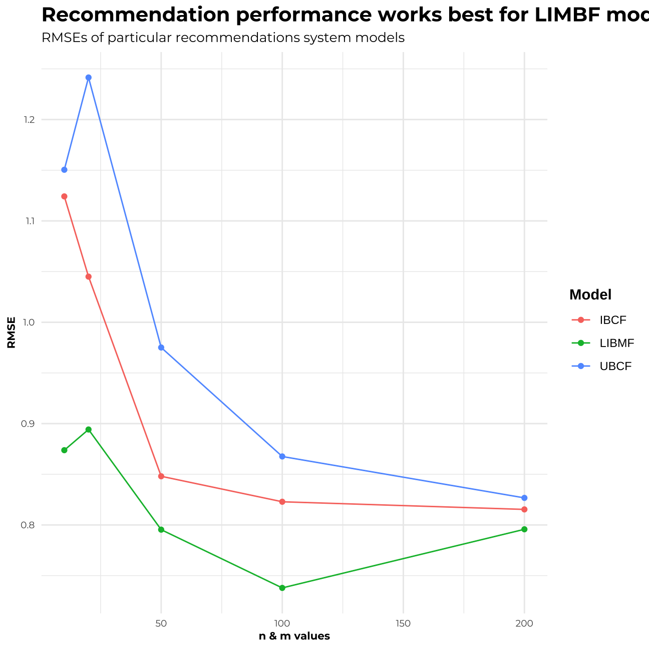
STEP 6 - CHOOSING THE OPTIMAL MODEL AND EVALUATING ITS RECOMMENDATIONS
From the above analysis, I can deduct that the best performing method and model I should choose for my recommendation system is the Matrix Factorisation Model with n & m= 100.
Such a model is based on the interactions between users and items. It is not only dependent on one of these variables. The big advantage is as well, that such a solution does not rely on the assumption of a large historical dataset. However, in the real world, such a model might not perform well for the rare movies. For these, we should try to use perhaps a different model of different m & n values and combine a mixed model that runs different analyses depending on the popularity of the movies and activeness of the users.
set.seed(1234) # setting seed
#this is our recommended model
recommen_model <- Recommender(getData(top100_split, "train"),
                              method = "LIBMF",
                              param=list(normalize = "center",
                                         method="Cosine"))
## Available parameter (with default values):
## dim = 10
## costp_l2 = 0.01
## costq_l2 = 0.01
## nthread = 1
## verbose = FALSEpredition_LIBMF <- predict(recommen_model, getData(top100_split, "known"), type="ratings")## iter tr_rmse obj
## 0 1.1885 2.0024e+04
## 1 0.8100 9.8797e+03
## 2 0.7955 9.5802e+03
## 3 0.7718 9.1092e+03
## 4 0.7498 8.6914e+03
## 5 0.7362 8.4326e+03
## 6 0.7270 8.2630e+03
## 7 0.7217 8.1623e+03
## 8 0.7170 8.0813e+03
## 9 0.7129 8.0064e+03
## 10 0.7096 7.9432e+03
## 11 0.7067 7.8942e+03
## 12 0.7036 7.8378e+03
## 13 0.7008 7.7878e+03
## 14 0.6980 7.7401e+03
## 15 0.6954 7.6948e+03
## 16 0.6924 7.6407e+03
## 17 0.6898 7.5953e+03
## 18 0.6869 7.5460e+03
## 19 0.6844 7.5028e+03#building a matrix
prediction_2 <- predict(recommen_model, top100_rate[1:25, ], type="ratings")## iter tr_rmse obj
## 0 1.1762 1.9580e+04
## 1 0.8039 9.7144e+03
## 2 0.7828 9.2965e+03
## 3 0.7584 8.8238e+03
## 4 0.7426 8.5223e+03
## 5 0.7323 8.3230e+03
## 6 0.7252 8.1958e+03
## 7 0.7206 8.1116e+03
## 8 0.7156 8.0203e+03
## 9 0.7120 7.9544e+03
## 10 0.7079 7.8818e+03
## 11 0.7046 7.8222e+03
## 12 0.7011 7.7617e+03
## 13 0.6974 7.6932e+03
## 14 0.6949 7.6527e+03
## 15 0.6911 7.5839e+03
## 16 0.6880 7.5297e+03
## 17 0.6850 7.4835e+03
## 18 0.6814 7.4205e+03
## 19 0.6785 7.3712e+03as(prediction_2, "matrix")[,1:10]## 356 318 296 593 2571 260 480 110 589 527
## [1,] NA NA NA NA NA NA NA NA NA NA
## [2,] NA NA NA NA NA NA NA NA NA 4.01
## [3,] NA NA NA NA NA NA NA NA NA NA
## [4,] NA 4.22 NA NA NA NA NA 3.77 NA 4.22
## [5,] NA NA NA NA NA NA NA NA NA NA
## [6,] NA NA NA NA NA NA NA NA NA NA
## [7,] NA NA NA NA NA NA NA NA NA NA
## [8,] NA NA NA NA NA NA NA NA NA 4.77
## [9,] NA NA NA NA NA NA NA NA NA NA
## [10,] NA NA NA NA NA NA NA NA NA NA
## [11,] NA NA NA NA NA NA NA NA NA NA
## [12,] NA NA NA NA NA NA NA NA NA 4.22
## [13,] NA NA NA NA NA NA NA NA NA NA
## [14,] NA NA NA NA NA NA NA NA NA NA
## [15,] NA 4.22 NA NA NA NA 2.76 NA 3.27 NA
## [16,] NA NA NA 3.48 NA NA NA NA NA 3.51
## [17,] NA NA NA NA NA NA NA 4.00 3.73 NA
## [18,] NA NA NA NA NA NA NA 3.79 3.63 NA
## [19,] NA NA NA 4.35 NA NA NA NA NA NA
## [20,] NA NA NA NA NA NA NA NA NA NA
## [21,] NA NA NA NA NA NA NA NA NA NA
## [22,] NA NA NA NA NA NA NA NA NA NA
## [23,] NA NA NA 4.60 NA NA NA NA NA NA
## [24,] NA NA NA NA NA NA NA NA NA NA
## [25,] NA NA NA NA NA NA 3.59 NA NA NA#finding recommended 5 movies for user 9
top100_rate[1,]## 1 x 134 rating matrix of class 'realRatingMatrix' with 133 ratings.recommended.items.u9<- predict(recommen_model, top100_rate[9,], n=5)## iter tr_rmse obj
## 0 1.2320 1.7357e+04
## 1 0.8243 8.2441e+03
## 2 0.8109 8.0137e+03
## 3 0.7990 7.8255e+03
## 4 0.7835 7.5721e+03
## 5 0.7702 7.3657e+03
## 6 0.7595 7.1981e+03
## 7 0.7505 7.0574e+03
## 8 0.7448 6.9676e+03
## 9 0.7384 6.8709e+03
## 10 0.7340 6.8041e+03
## 11 0.7292 6.7305e+03
## 12 0.7252 6.6733e+03
## 13 0.7213 6.6139e+03
## 14 0.7176 6.5630e+03
## 15 0.7143 6.5117e+03
## 16 0.7110 6.4643e+03
## 17 0.7076 6.4154e+03
## 18 0.7047 6.3734e+03
## 19 0.7017 6.3311e+03as(recommended.items.u9, "list")[[1]]## [1] "4878" "608" "1073" "1213" "68954"# [1] "608" "1213" "4878" "1265" "1197" movieIDs
movies_u9<- c()
movies_u9<- append(movies_u9,movie_data$title[movie_data$movieId %in% "608"])
# "Fargo (1996)"
movies_u9<- append(movies_u9,movie_data$title[movie_data$movieId %in% "1213"])
# "Goodfellas (1990)"
movies_u9<- append(movies_u9,movie_data$title[movie_data$movieId %in% "4878"])
# "Donnie Darko (2001)"
movies_u9<- append(movies_u9,movie_data$title[movie_data$movieId %in% "1265"])
# "Groundhog Day (1993)"
movies_u9<- append(movies_u9,movie_data$title[movie_data$movieId %in% "1197"])
# "Princess Bride, The (1987)"
movies_u9## [1] "Fargo (1996)" "Goodfellas (1990)"
## [3] "Donnie Darko (2001)" "Groundhog Day (1993)"
## [5] "Princess Bride, The (1987)"— END —
