Interest rate analysis in R using logistic models
Introduction
I will continue working with the lending club data.
I will take the perspective of an investor to the lending club.
The goal is to select a subset of the most promising loans to invest. I will do so using the method of logistic regression.
Load the data
lc_raw <- read_csv("~/Documents/LBS/Data Science/Session 03/LendingClub Data.csv",  skip=1) %>%  #since the first row is a title we want to skip it.
  clean_names() # use janitor::clean_names()
ICE the data: Inspect, Clean, Explore
Any data science engagement starts with ICE. Inspecting, Clean and Explore the data.
Inspect the data
I will inspect the data to understand what different variables mean.
summary(lc_raw)## int_rate loan_amnt term_months installment dti
## Min. :0 Min. : 500 Min. :36 Min. : 16 Min. : 0
## 1st Qu.:0 1st Qu.: 5500 1st Qu.:36 1st Qu.: 169 1st Qu.: 8
## Median :0 Median :10000 Median :36 Median : 288 Median :13
## Mean :0 Mean :11253 Mean :42 Mean : 333 Mean :13
## 3rd Qu.:0 3rd Qu.:15000 3rd Qu.:60 3rd Qu.: 449 3rd Qu.:19
## Max. :0 Max. :35000 Max. :60 Max. :1305 Max. :30
## NA's :4669 NA's :4669 NA's :4669 NA's :4669 NA's :4669
## delinq_2yrs annual_inc grade emp_title
## Min. : 0 Min. : 4000 Length:42538 Length:42538
## 1st Qu.: 0 1st Qu.: 40800 Class :character Class :character
## Median : 0 Median : 59534 Mode :character Mode :character
## Mean : 0 Mean : 69148
## 3rd Qu.: 0 3rd Qu.: 82800
## Max. :11 Max. :6000000
## NA's :4669 NA's :4669
## emp_length home_ownership verification_status issue_d
## Length:42538 Length:42538 Length:42538 Length:42538
## Class :character Class :character Class :character Class :character
## Mode :character Mode :character Mode :character Mode :character
##
##
##
##
## zip_code addr_state loan_status desc
## Length:42538 Length:42538 Length:42538 Length:42538
## Class :character Class :character Class :character Class :character
## Mode :character Mode :character Mode :character Mode :character
##
##
##
##
## purpose title x20 x21
## Length:42538 Length:42538 Mode:logical Mode:logical
## Class :character Class :character NA's:42538 NA's:42538
## Mode :character Mode :character
##
##
##
##
## x22 x23 x24 x25 x26
## Mode:logical Mode:logical Mode:logical Mode:logical Mode:logical
## NA's:42538 NA's:42538 NA's:42538 NA's:42538 NA's:42538
##
##
##
##
##
## x27 x28 x29 x30 x31
## Mode:logical Mode:logical Mode:logical Mode:logical Mode:logical
## NA's:42538 NA's:42538 NA's:42538 NA's:42538 NA's:42538
##
##
##
##
##
## x32 x33 x34 x35 x36
## Mode:logical Mode:logical Mode:logical Mode:logical Mode:logical
## NA's:42538 NA's:42538 NA's:42538 NA's:42538 NA's:42538
##
##
##
##
##
## x37 x38 x39 x40 x41
## Mode:logical Mode:logical Mode:logical Mode:logical Mode:logical
## NA's:42538 NA's:42538 NA's:42538 NA's:42538 NA's:42538
##
##
##
##
##
## x42 x43 x44 x45 x46
## Mode:logical Mode:logical Mode:logical Mode:logical Mode:logical
## NA's:42538 NA's:42538 NA's:42538 NA's:42538 NA's:42538
##
##
##
##
##
## x47 x48 x49 x50 x51
## Mode:logical Mode:logical Mode:logical Mode:logical Mode:logical
## NA's:42538 NA's:42538 NA's:42538 NA's:42538 NA's:42538
##
##
##
##
##
## x52 x53 x54 x55 x56
## Mode:logical Mode:logical Mode:logical Mode:logical Mode:logical
## NA's:42538 NA's:42538 NA's:42538 NA's:42538 NA's:42538
##
##
##
##
##
## x57 x58 x59 x60 x61
## Mode:logical Mode:logical Mode:logical Mode:logical Mode:logical
## NA's:42538 NA's:42538 NA's:42538 NA's:42538 NA's:42538
##
##
##
##
##
## x62 x63 x64 x65 x66
## Mode:logical Mode:logical Mode:logical Mode:logical Mode:logical
## NA's:42538 NA's:42538 NA's:42538 NA's:42538 NA's:42538
##
##
##
##
##
## x67 x68 x69 x70 x71
## Mode:logical Mode:logical Mode:logical Mode:logical Mode:logical
## NA's:42538 NA's:42538 NA's:42538 NA's:42538 NA's:42538
##
##
##
##
##
## x72 x73 x74 x75 x76
## Mode:logical Mode:logical Mode:logical Mode:logical Mode:logical
## NA's:42538 NA's:42538 NA's:42538 NA's:42538 NA's:42538
##
##
##
##
##
## x77 x78 x79 x80
## Mode:logical Mode:logical Mode :logical Mode :logical
## NA's:42538 NA's:42538 FALSE:2660 FALSE:2718
## NA's :39878 NA's :39820
##
##
##
## Clean the data
Are there any redundant columns and rows? Are all the variables in the correct format (e.g., numeric, factor, date)? Lets fix it.
The variable “loan_status” contains information as to whether the loan has been repaid or charged off (i.e., defaulted). I will create a binary factor variable for this and focus on it in my further analysis.
lc_clean<- lc_raw %>%
  dplyr::select(-x20:-x80) %>% #delete empty columns
  filter(!is.na(int_rate)) %>%   #delete empty rows
  mutate(
    issue_d = lubridate::mdy(issue_d),  # lubridate::mdy() to fix date format
    term = factor(term_months),     # turn 'term' into a categorical variable
    delinq_2yrs = factor(delinq_2yrs) # turn 'delinq_2yrs' into a categorical variable
  ) %>%
  mutate(default = dplyr::recode(loan_status,
                      "Charged Off" = "1",
                      "Fully Paid" = "0"))%>%
    mutate(default = as.factor(default)) %>%
  dplyr::select(-emp_title,-installment, -term_months, everything()) #move some not-so-important variables to the end.
Explore the data
I will explore loan defaults by creating different visualizations. I will start with examining how prevalent defaults are, whether the default rate changes by loan grade or number of delinquencies, and a couple of scatter plots of defaults against loan amount and income.
#bar chart of defaults
def_vis1<-ggplot(data=lc_clean, aes(x=default)) +
  geom_bar(aes(y = (..count..)/sum(..count..))) +
  labs(x="Default, 1=Yes, 0=No", y="relative frequencies") +
  scale_y_continuous(labels=scales::percent) +
  geom_text(aes( label = scales::percent((..count..)/sum(..count..) ),y=(..count..)/sum(..count..) ), stat= "count",vjust=-0.5)

def_vis1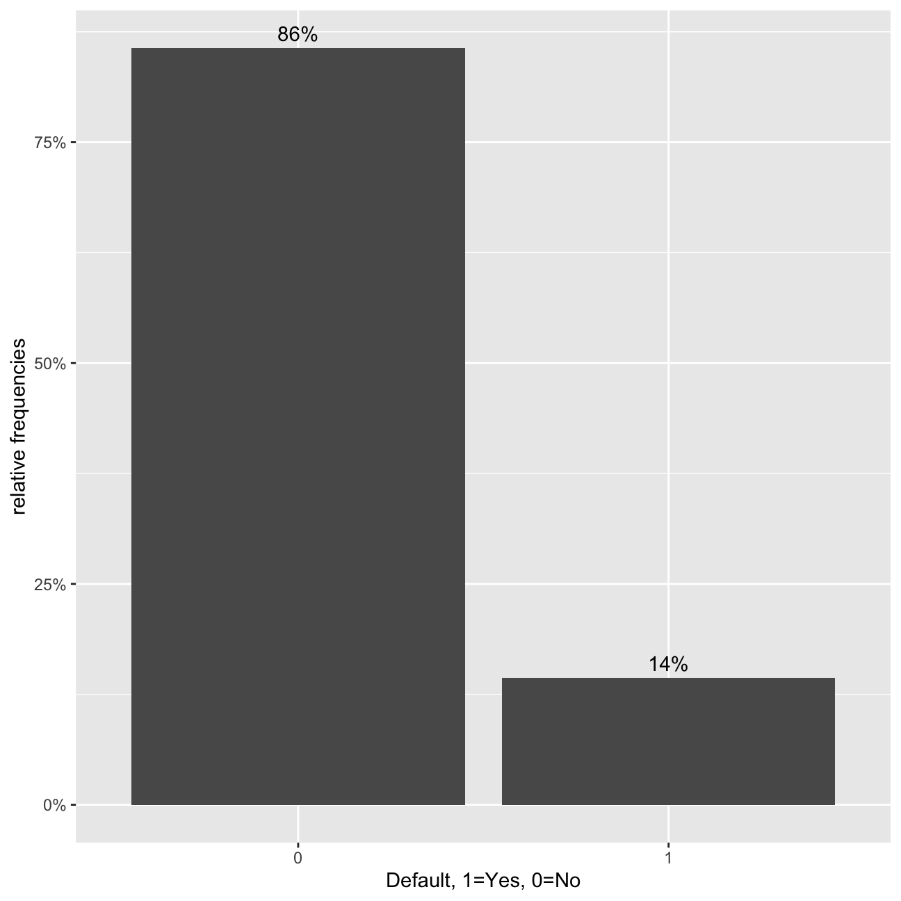
#bar chart of defaults per loan grade
def_vis2<-ggplot(data=lc_clean, aes(x=default), group=grade) +
  geom_bar(aes(y = (..count..)/sum(..count..), fill = factor(..x..)), stat="count")  +
  labs(title="Defaults by Grade", x="Default, 1=Yes, 0=No", y="relative frequencies") +
  scale_y_continuous(labels=scales::percent) +facet_grid(~grade) +
  theme(legend.position = "none") +
  geom_text(aes( label = scales::percent((..count..)/sum(..count..) ),y=(..count..)/sum(..count..) ), stat= "count",vjust=-0.5)

def_vis2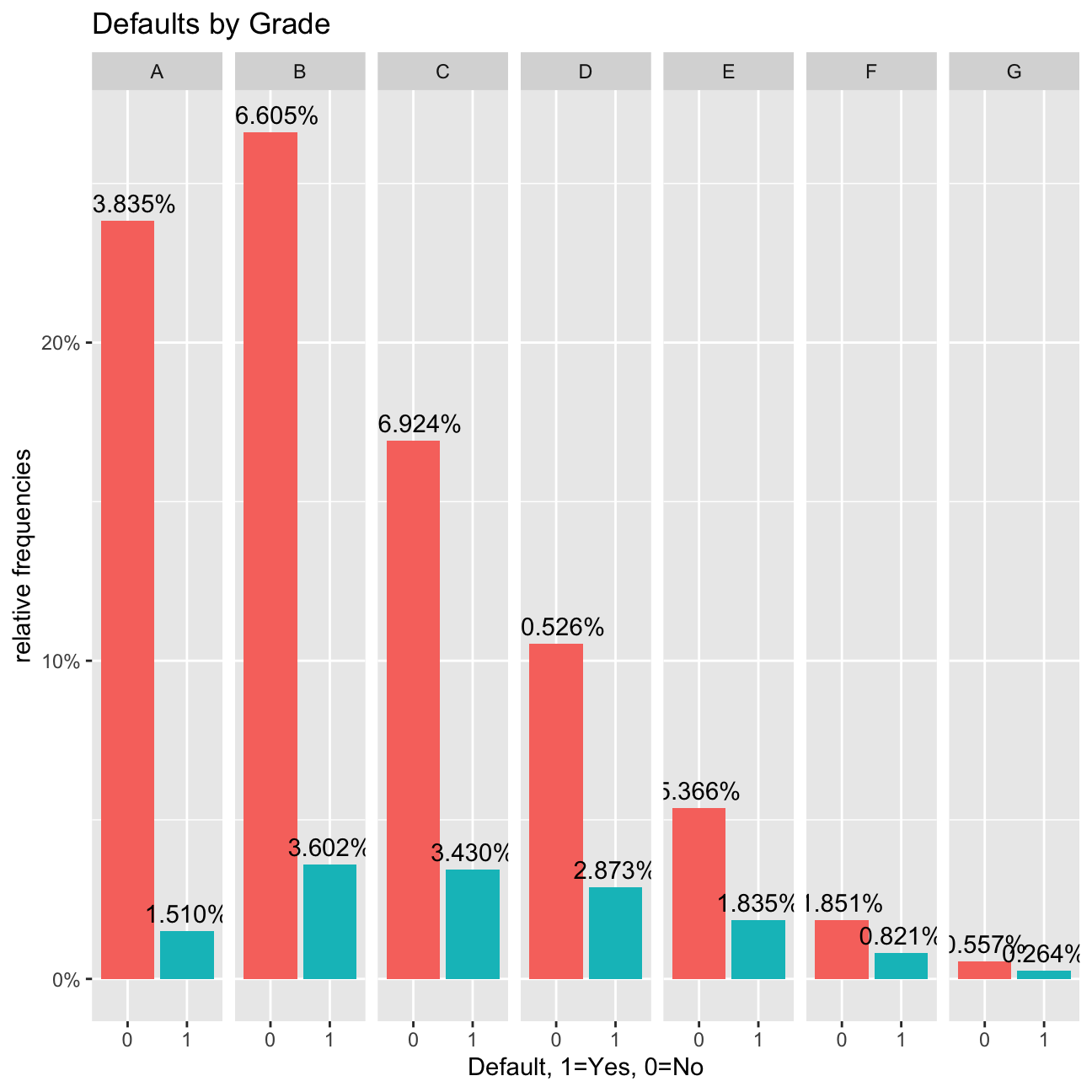
#bar chart of defaults per number of Delinquencies
def_vis3<-lc_clean %>%
  filter(as.numeric(delinq_2yrs)<4) %>%
  ggplot(aes(x=default), group=delinq_2yrs) +
  geom_bar(aes(y = (..count..)/sum(..count..), fill = factor(..x..)), stat="count")  +
  labs(title="Defaults by Number of Delinquencies", x="Default, 1=Yes, 0=No", y="relative frequencies") +
  scale_y_continuous(labels=scales::percent) +
  facet_grid(~delinq_2yrs) +
  theme(legend.position = "none") +
  geom_text(aes( label = scales::percent((..count..)/sum(..count..) ),y=(..count..)/sum(..count..) ), stat= "count",vjust=-0.5)

def_vis3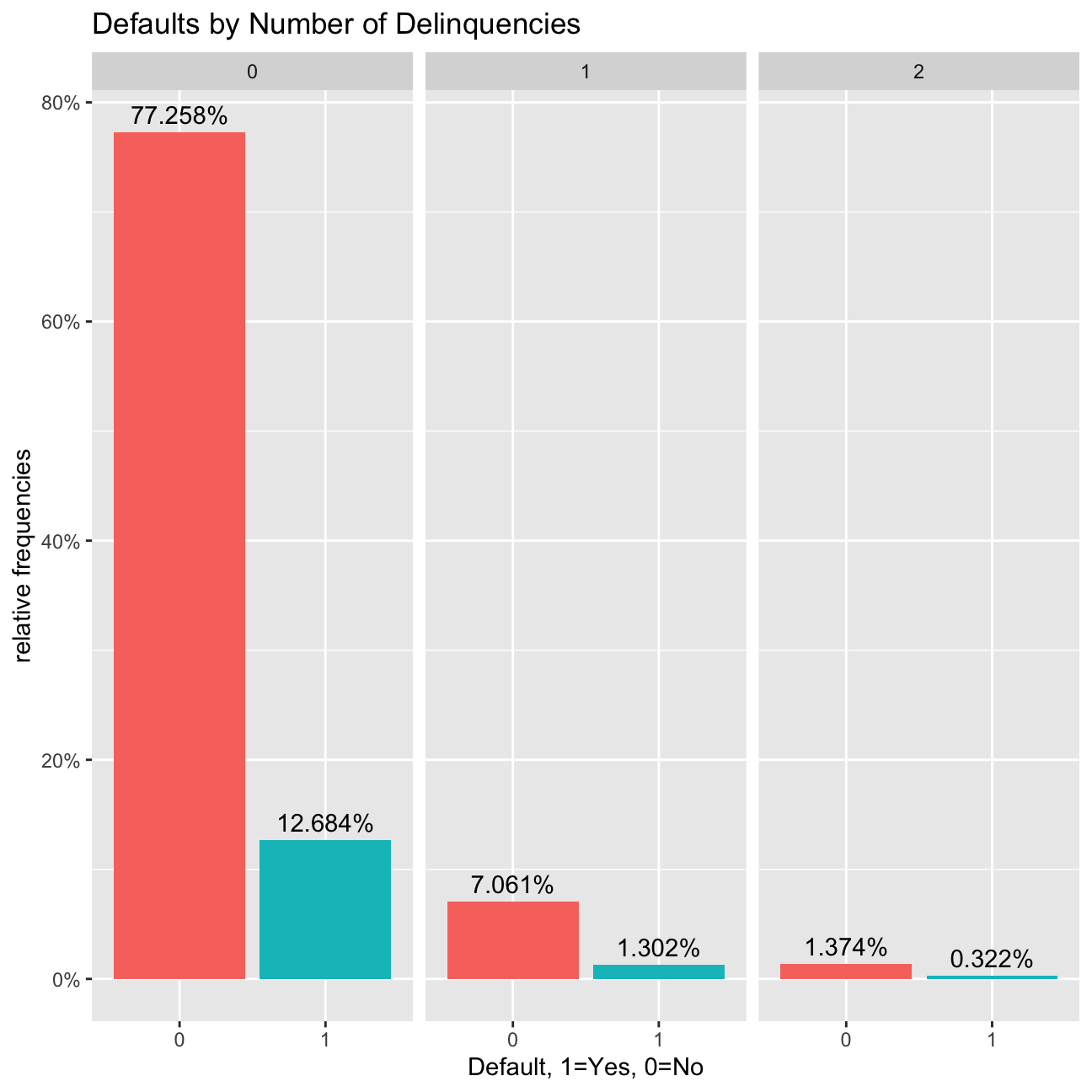
#scatter plots

#We select 2000 random loans to display only to make the display less busy.
set.seed(1234)
reduced<-lc_clean[sample(0:nrow(lc_clean), 2000, replace = FALSE),]%>%
  mutate(default=as.numeric(default)-1) # also convert default to a numeric {0,1} to make it easier to plot.


# scatter plot of defaults against loan amount
def_vis4<-ggplot(data=reduced, aes(y=default,x=I(loan_amnt/1000)))  +
  labs(y="Default, 1=Yes, 0=No", x="Loan Amnt (1000 $)") +
  geom_jitter(width=0, height=0.05, alpha=0.7)

def_vis4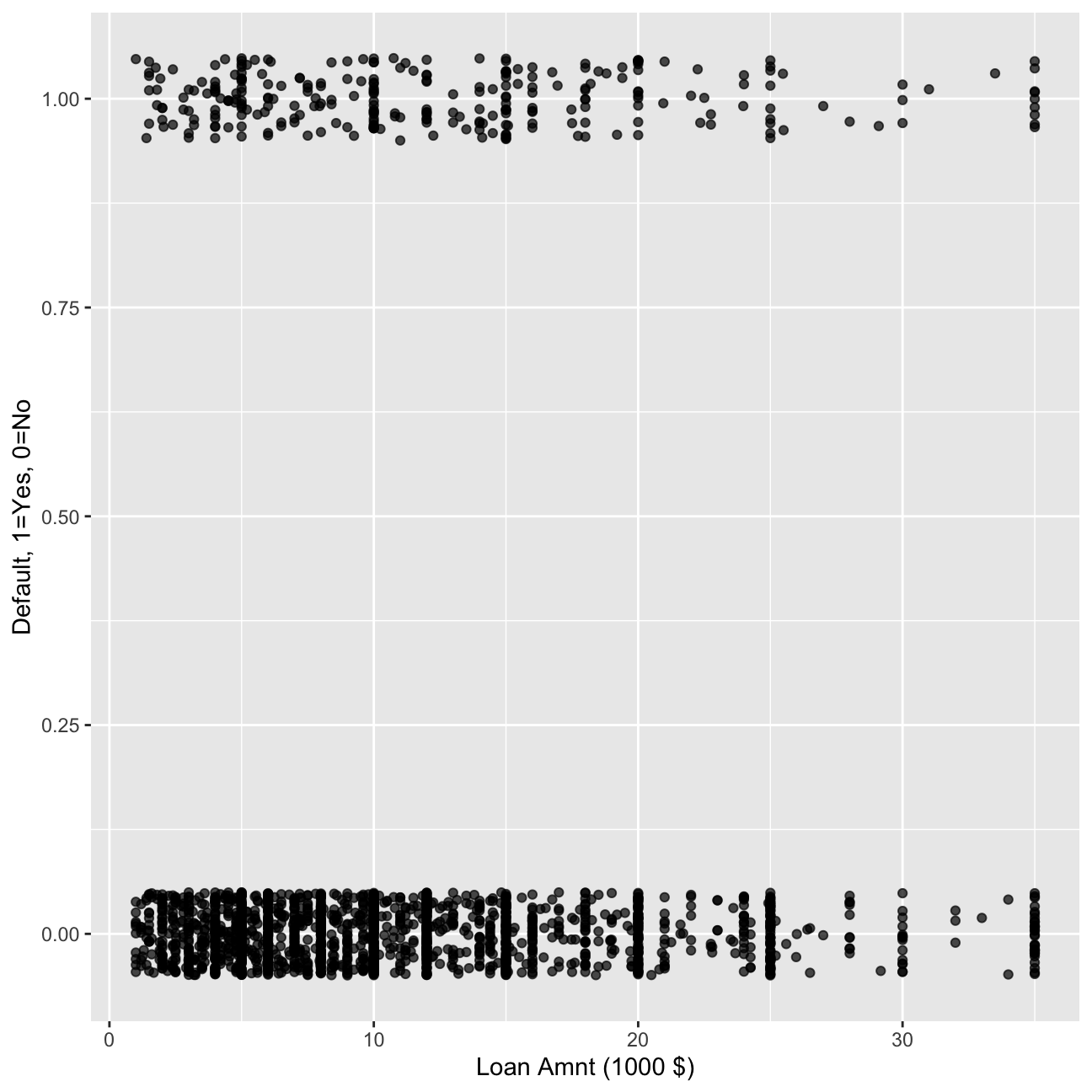
#scatter plot of defaults against loan amount.
def_vis5<-ggplot(data=reduced, aes(y=default,x=I(annual_inc/1000))) +
  labs(y="Default, 1=Yes, 0=No", x="Annual Income(1000 $)") +
  geom_jitter(width=0, height=0.05, alpha=0.7) +
  xlim(0,400)

def_vis5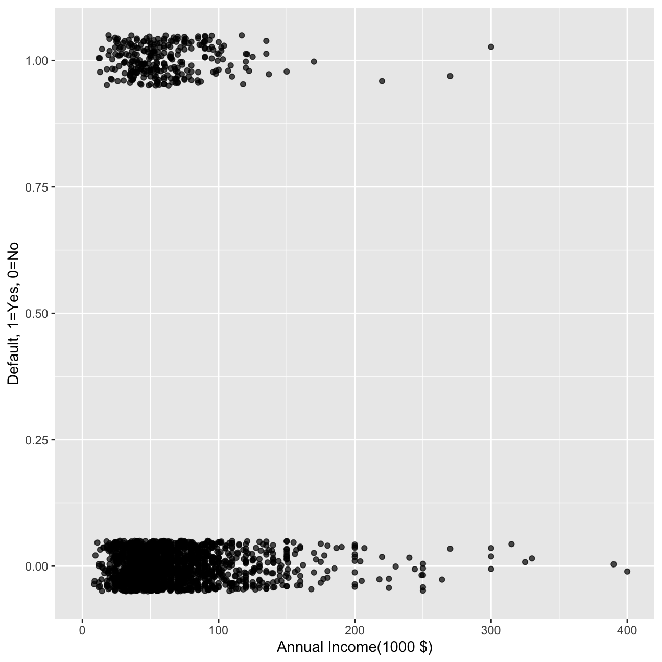
I will also estimate a correlation table between defaults and other continuous variables.
# correlation table using GGally::ggcor()
# this takes a while to plot
lc_clean %>%
    mutate(default=as.numeric(default)-1)%>%
  select(loan_amnt, dti, annual_inc, default) %>% #keep Y variable last
 ggcorr(method = c("pairwise", "pearson"), label_round=2, label = TRUE)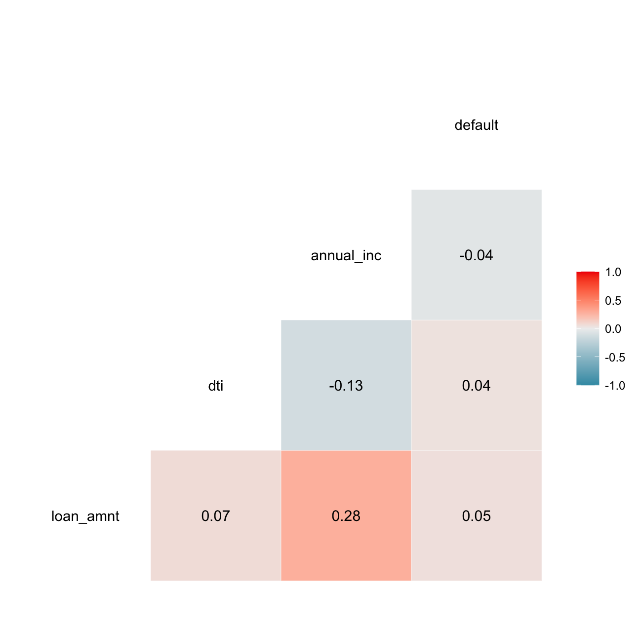
ggplot(lc_clean, aes(x= loan_amnt,y= default, colour=term)) +
  geom_boxplot() +
  facet_wrap(~grade) +
  labs(title= "Average annual income across all the grades for term 36 and 60", y="Default", x="Annual Income(1000 $)")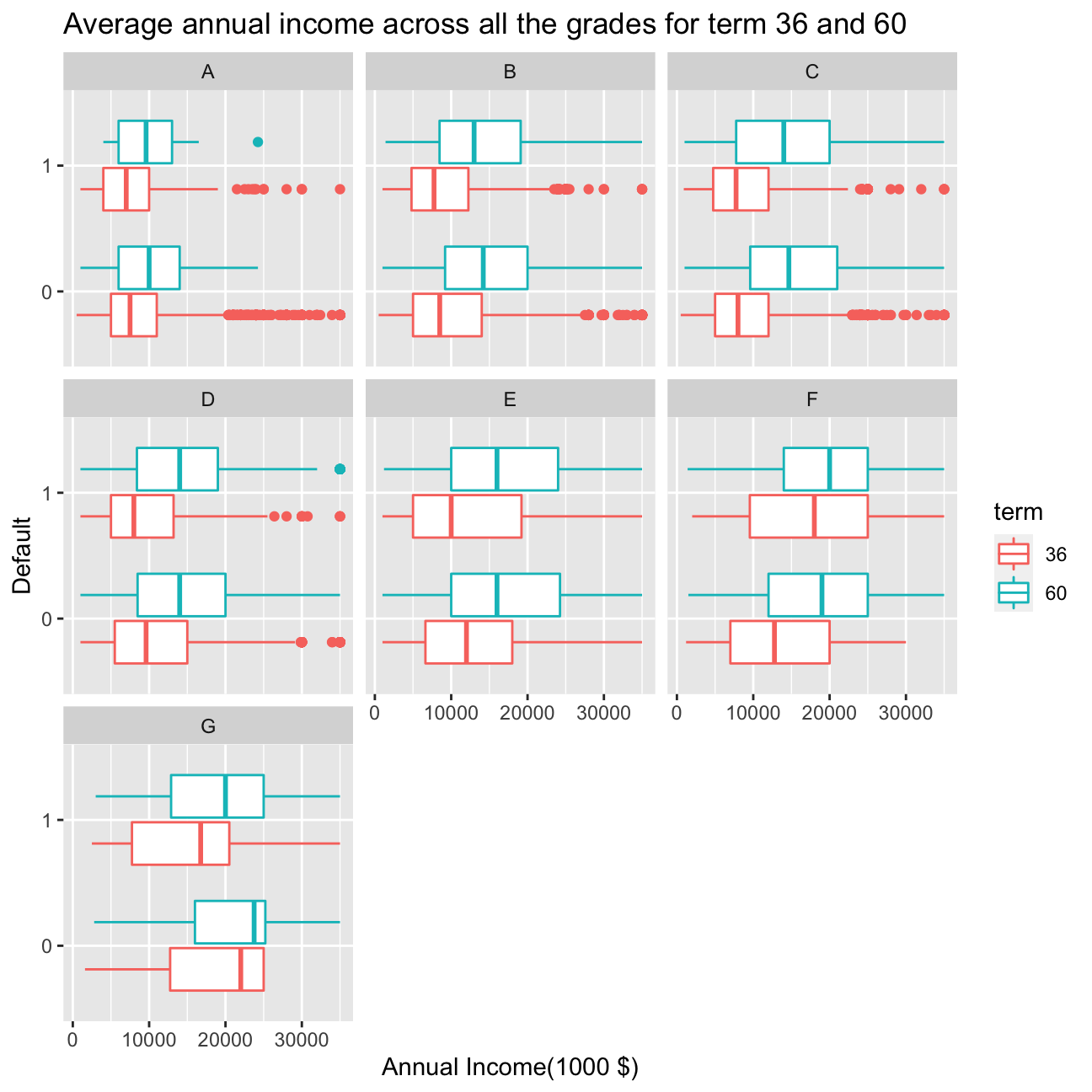
lc_clean %>%
  select(grade, int_rate, default) %>%
           ggpairs(aes(colour=default), alpha=1)+
  theme_bw()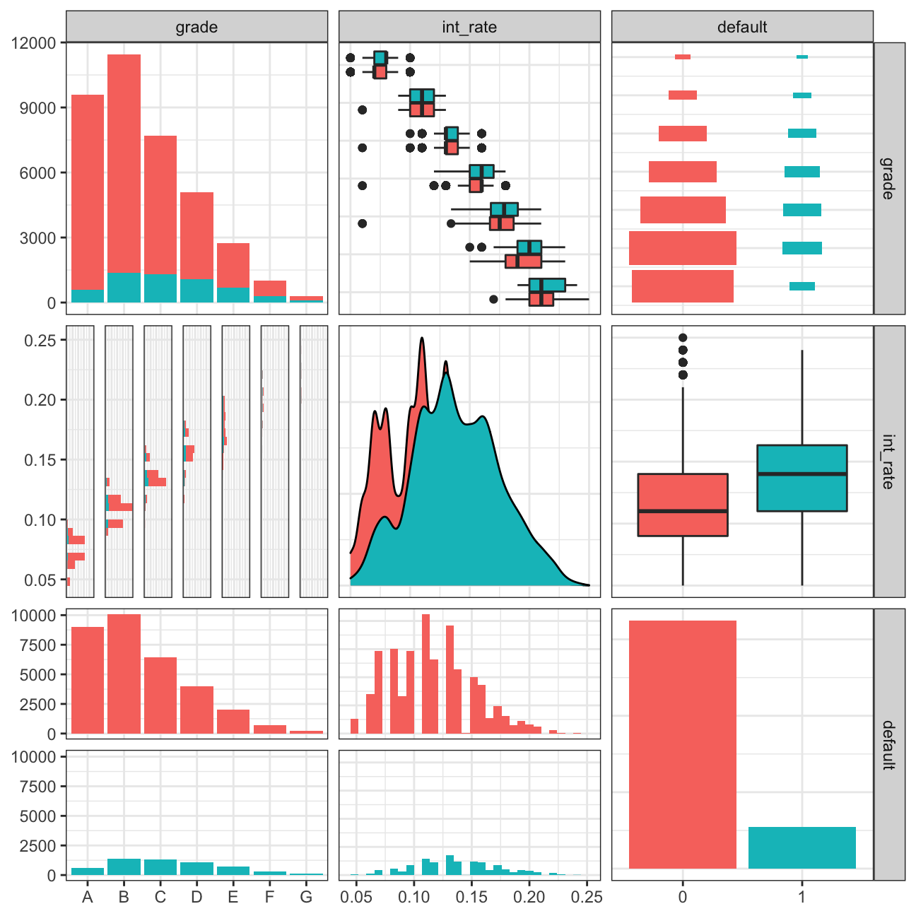
From the graph it is interesting to observe that across particular loan grades from A to G the loan amount tends to increase in both terms for 36 months and 60 months. However, the loan amount for 36 months always stays slower disregard grade or default.
From the ggpairs plot, we can draw a few conclusions. First of all, the amount of data on default=1 is much smaller than the smount of data on default=0. Second of all, the biggest group by grade is group B, and groups that mostly tend to default are B, C or D. Interestingly, the interest rate tends to be bigger for people who fail to pay the loan back. Also the interest rate is the lowest for grade A and increases across the grades.
Linear vs. logistic regression for binary response variables
It is certainly possible to use the OLS approach to find the line that minimizes the sum of square errors when the dependent variable is binary (i.e., default no default). In this case, the predicted values take the interpretation of a probability. I can also estimate a logistic regression instead. I will do both below.
model_lm<-lm(as.numeric(default)~I(annual_inc/1000), lc_clean)
summary(model_lm)
##
## Call:
## lm(formula = as.numeric(default) ~ I(annual_inc/1000), data = lc_clean)
##
## Residuals:
## Min 1Q Median 3Q Max
## -0.160 -0.149 -0.144 -0.133 1.327
##
## Coefficients:
## Estimate Std. Error t value Pr(>|t|)
## (Intercept) 1.16e+00 2.70e-03 429.3 <2e-16 ***
## I(annual_inc/1000) -2.48e-04 2.92e-05 -8.5 <2e-16 ***
## ---
## Signif. codes: 0 '***' 0.001 '**' 0.01 '*' 0.05 '.' 0.1 ' ' 1
##
## Residual standard error: 0.35 on 37867 degrees of freedom
## Multiple R-squared: 0.0019, Adjusted R-squared: 0.00188
## F-statistic: 72.2 on 1 and 37867 DF, p-value: <2e-16logistic1<-glm(default~I(annual_inc/1000), family="binomial", lc_clean)
summary(logistic1)##
## Call:
## glm(formula = default ~ I(annual_inc/1000), family = "binomial",
## data = lc_clean)
##
## Deviance Residuals:
## Min 1Q Median 3Q Max
## -0.625 -0.579 -0.557 -0.511 3.639
##
## Coefficients:
## Estimate Std. Error z value Pr(>|z|)
## (Intercept) -1.51916 0.02924 -52.0 <2e-16 ***
## I(annual_inc/1000) -0.00408 0.00040 -10.2 <2e-16 ***
## ---
## Signif. codes: 0 '***' 0.001 '**' 0.01 '*' 0.05 '.' 0.1 ' ' 1
##
## (Dispersion parameter for binomial family taken to be 1)
##
## Null deviance: 31130 on 37868 degrees of freedom
## Residual deviance: 31005 on 37867 degrees of freedom
## AIC: 31009
##
## Number of Fisher Scoring iterations: 5ggplot(data=reduced, aes(x=I(annual_inc/1000), y=default)) +
geom_smooth(method="lm", se=0, aes(color="OLS"))+ geom_smooth(method = "glm", method.args = list(family = "binomial"), se=0, aes(color="Logistic")) +
labs(y="Prob of Default", x="Annual Income(1000 $)") + xlim(0,450)+scale_y_continuous(labels=scales::percent) +
geom_jitter(width=0, height=0.05, alpha=0.7) +
scale_colour_manual(name="Fitted Model", values=c("blue", "red"))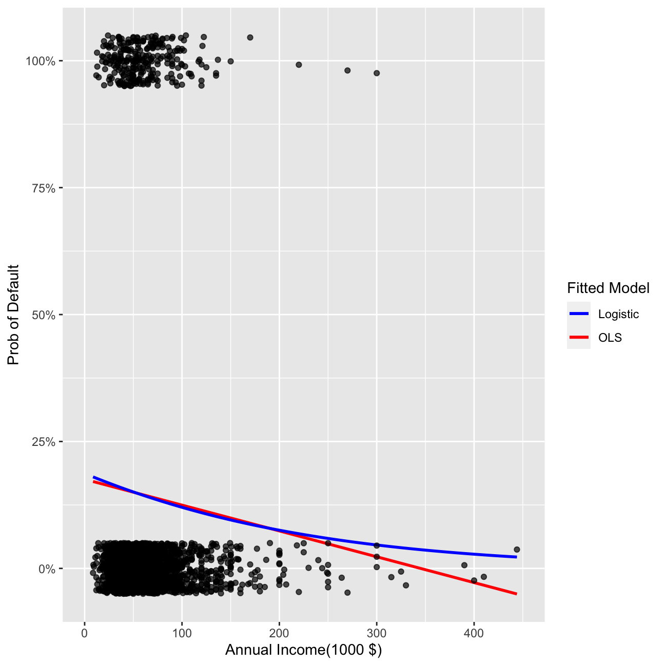
Conclusion
Logistic model in the case when real y (default) takes values equal to 0 or 1 is much better than OLS. It is because it avoids the negative values for probability, which are impossible to achieve empirically and not explainable.
Multivariate logistic regression
I can estimate logistic regression with multiple explanatory variables as well. For that, I will use annual_inc, term, grade, and loan amount as features.
logistic2<-glm(default~I(annual_inc/1000)+term+grade+loan_amnt, family="binomial", lc_clean)
summary(logistic2)
##
## Call:
## glm(formula = default ~ I(annual_inc/1000) + term + grade + loan_amnt,
## family = "binomial", data = lc_clean)
##
## Deviance Residuals:
## Min 1Q Median 3Q Max
## -1.063 -0.608 -0.482 -0.345 4.099
##
## Coefficients:
## Estimate Std. Error z value Pr(>|z|)
## (Intercept) -2.43e+00 5.06e-02 -48.09 <2e-16 ***
## I(annual_inc/1000) -6.02e-03 4.73e-04 -12.73 <2e-16 ***
## term60 4.79e-01 3.56e-02 13.45 <2e-16 ***
## gradeB 6.60e-01 5.27e-02 12.52 <2e-16 ***
## gradeC 1.03e+00 5.39e-02 19.13 <2e-16 ***
## gradeD 1.29e+00 5.70e-02 22.58 <2e-16 ***
## gradeE 1.42e+00 6.66e-02 21.24 <2e-16 ***
## gradeF 1.67e+00 8.63e-02 19.30 <2e-16 ***
## gradeG 1.77e+00 1.34e-01 13.20 <2e-16 ***
## loan_amnt 2.84e-06 2.35e-06 1.21 0.23
## ---
## Signif. codes: 0 '***' 0.001 '**' 0.01 '*' 0.05 '.' 0.1 ' ' 1
##
## (Dispersion parameter for binomial family taken to be 1)
##
## Null deviance: 31130 on 37868 degrees of freedom
## Residual deviance: 29286 on 37859 degrees of freedom
## AIC: 29306
##
## Number of Fisher Scoring iterations: 5#compare the fit of logistic 1 and logistic 2
anova(logistic1,logistic2)| Resid. Df | Resid. Dev | Df | Deviance |
|---|---|---|---|
| 3.79e+04 | 3.1e+04 | ||
| 3.79e+04 | 2.93e+04 | 8 | 1.72e+03 |
Explanation of the notions:
Estimated Coefficient The Estimated Coeffiecient explains how a change in a particular varaible influence directly the risk factor decrease/increase. Risk factor is connected to the outcome y (probability) though the logistic function in the model. Sign of the coefficient has a general interpretation - if negative, the change in variable by 1 will cause decrease in the probability. If coeffiecient is positive, the change in variable by 1 will cause increase in probability.
Standard error of coefficient The magnitude of the standard error estimates how estimated coefficient would be affected if different data are fed in the model. It is also useful when constructing the 95% Confidence Interval for the true coefficients.
p-value of coefficient The p-value of the coefficient is connected to the Z-score in the Z-test. If the p-value is smaller than 0.05, the coeffieint is signifficant. The p-value describes the probability of the coeffiecient’s value falling inside the 95% confidence interval.
Deviance Deviance (or -2 log-likelihood (-2LL) statistic) is a goodness-of-fit statistic for a statistical model. We often use it for statistical hypothesis testing. Deviance is a generalization of the idea of using the sum of squares of residuals in ordinary least squares to cases where model-fitting is achieved by maximum likelihood. It tells us how much unexplained variation there is in our logistic regression model - the higher the value the less accurate the model.
AIC The Akaike Information Critetion rectifies deviance by penalizing number of coefficients. In other words AIC is an estimator of out-of-sample prediction error. The furmula is as follows: =-2log(L)+2k, where k is the number of coefficients. Again, the lower the score, the more accurate our model. AIC is used most frequently in situations when one is not able to easilty test model’s performance with use of machine learning (when having a small dataset or time series).
Null Deviance It is the outcome of Deviance, when model depends only on intercept.
Conclusion
FOr our predicitons, logistic 2 model is better than logistic 1 model as both deviance and AIC are lower.
Predicting probability
#Predict the probability of default
prob_default2<-predict(logistic2, lc_clean, type="response")

#plot 1: Density of predictions
g0<-ggplot( lc_clean, aes( prob_default2 ) )+
  geom_density( size=1)+
  ggtitle( "Predicted Probability with Logistic 2" )+  xlab("Estimated Probability")
g0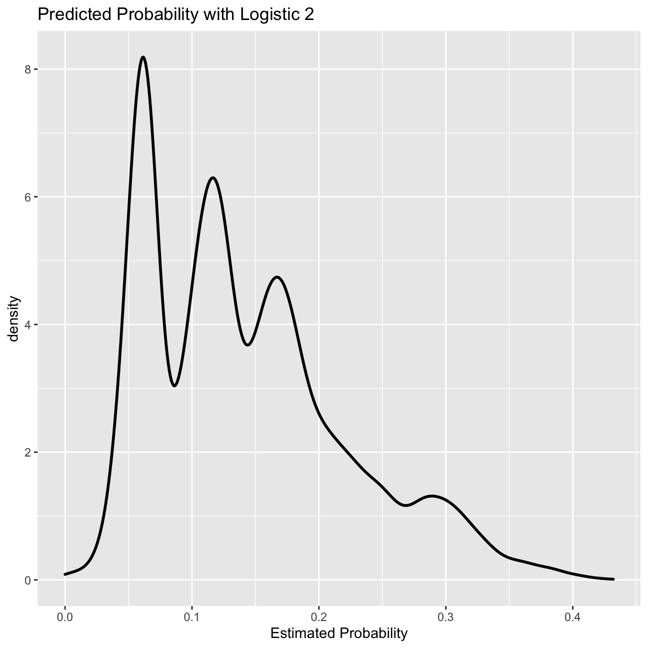
#plot 2: Density of predictions by default
g1<-ggplot( lc_clean, aes( prob_default2, color=default) ) +
  geom_density( size=1)+
  ggtitle( "Predicted Probability with Logistic 2 by default" )+  xlab("Estimated Probability")
g1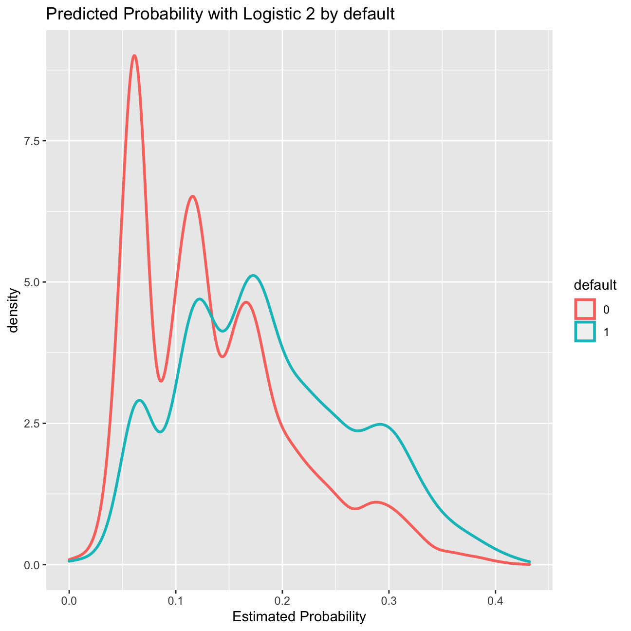
From probability to classification
The logistic regression model gives us a sense of how likely defaults are; it gives us a probability estimate. To convert this into a prediction, we need to choose a cutoff probability and classify every loan with a predicted probability of default above the cutoff as a prediction of default (and vice versa for loans with a predicted probability below this cutoff).
Let’s choose a threshold of 20%. Of course some of our predictions will turn out to be right but some will turn out to be wrong – you can see this in the density figures of the previous section. Let’s call “default” the “positive” class since this is the class we are trying to predict. We could be making two types of mistakes. False positives (i.e., predict that a loan will default when it will not) and false negatives (I.e., predict that a loan will not default when it does). These errors are summarized in the confusion matrix.
Confusion matrix
I will now produce the confusion matrix for the model logistic 2 for a cutoff of 18%.
#using the logistic 2 model predict default probabilities
prob_default2<- predict(logistic2, lc_clean, type="response")

#Call any loan with probability more than 18% as default and any loan with lower probability as non-default.
p_class<-factor(ifelse(prob_default2>0.18,"1","0"),levels=levels(lc_clean$default))

#produce the confusion matrix and set default as the positive outcome
con2<-confusionMatrix(p_class,lc_clean$default,positive="1")

#print the confusion matrix
con2
## Confusion Matrix and Statistics
##
## Reference
## Prediction 0 1
## 0 24674 2818
## 1 7766 2611
##
## Accuracy : 0.721
## 95% CI : (0.716, 0.725)
## No Information Rate : 0.857
## P-Value [Acc > NIR] : 1
##
## Kappa : 0.175
##
## Mcnemar's Test P-Value : <2e-16
##
## Sensitivity : 0.4809
## Specificity : 0.7606
## Pos Pred Value : 0.2516
## Neg Pred Value : 0.8975
## Prevalence : 0.1434
## Detection Rate : 0.0689
## Detection Prevalence : 0.2740
## Balanced Accuracy : 0.6208
##
## 'Positive' Class : 1
## Using the confusion matrix, I can calculate the following:
a. Accuracy
Percentage of status correctly predicted, regardless of default status.
(2611+24674)/(2611+2818+24674+7766)=0.7205
b. Sensitivity
Proportion of good loans correctly identified as non-default.
2611/(2611+2818)=0.48094
c. Specificity
Proportion of bad loans correctly identified as default.
24674/(24674+7766)=0.76060
ROC curve and AUS
Using the model logistic 2 I will produce the ROC curve and calculate the AUC measure.
#estimate the ROC curve for Logistic 2
ROC_logistic2 <- roc(lc_clean$default,prob_default2)

#estimate the AUC for Logistic 2 and round it to two decimal places
AUC2<-round(auc(lc_clean$default,prob_default2)*100, digits=2)
#Plot the ROC curve and display the AUC in the title
ROC2<-ggroc(ROC_logistic2,  alpha = 0.5)+ ggtitle(paste("Model Logistic 2: AUC=",round(auc(lc_clean$default,prob_default2)*100, digits=2),"%"))  + geom_segment(aes(x = 1, xend = 0, y = 0, yend = 1), color="grey", linetype="dashed")+geom_segment(aes(x = 1, xend = 1, y = 0, yend = 1), color="black", linetype="dashed")+geom_segment(aes(x = 1, xend = 0, y = 1, yend = 1), color="black", linetype="dashed")

ROC2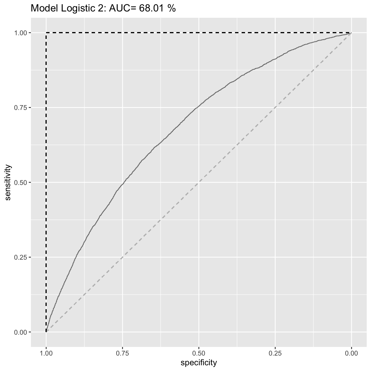
The ROC curve shows for any given level of True Positives, what level of True Negatives we can expect.The stright line shows the situation in which instead of a model we were using the probability of 0.5. Anything about the line is better than the random prediction. We aim for the ROC to be as close to the (1.00,1.00) point as possible. The AUC measure measures the area under the curve. Again for random prediciton (stright line) the AUC=0.5. The better the AUC the better the model. We expect the AUC of any predictive model to be between 0.5 and 1 as we expect is to be better than the random prediciton based on 0.5 chance. In case of a bad model, the AUC could be equal to the number below 0.5. However, in that case, we should immediately drop the model, as it means, that our model predictions are worse that the random chance of being correct. The AUC cannot be equal to the number above 1, as in case AUC=1, the model predictions are already 100% correct.
Out of sample ROC curve estimation
So far we have only worked in-sample. I will now split the data into training and testing and estimate the models ROC curve and AUC measure out of sample.
# splitting the data into training and testing
set.seed(1234)
train_test_split <- initial_split(lc_clean, prop = 0.8)
testing <- testing(train_test_split) #20% of the data is set aside for testing
training <- training(train_test_split) #80% of the data is set aside for training

# run logistic 2 on the training set
logistic2_in<-glm(default~I(annual_inc/1000)+term+grade+loan_amnt, family="binomial", training)

#calculate probability of default in the training sample
p_in<-predict(logistic2_in, training, type = "response")

#ROC curve using in-sample predictions
ROC_logistic2_in <- roc(training$default,p_in)
#AUC using in-sample predictions
AUC_logistic2_in<-round(auc(training$default,p_in)*100, digits=2)

#calculate probability of default out of sample
p_out<-predict(logistic2_in, testing, type = "response")

#ROC curve using out-of-sample predictions
ROC_logistic2_out <- roc(testing$default,p_out)
#AUC using out-of-sample predictions
AUC_logistic2_out <- round(auc(testing$default,p_out)*100, digits=2)
#plot in the same figure both ROC curves and print the AUC of both curves in the title
ggroc(list("Logistic 2 in-sample"=ROC_logistic2_in, "Logistic 2 out-of-sample"=ROC_logistic2_out))+ggtitle(paste("Model Logistic 2 in-sample AUC=",round(auc(training$default,p_in)*100, digits=2),"%\nModel Logistic 2 out-of-sample AUC=",round(auc(testing$default,p_out)*100, digits=2),"%"))    +
geom_segment(aes(x = 1, xend = 0, y = 0, yend = 1), color="grey", linetype="dashed")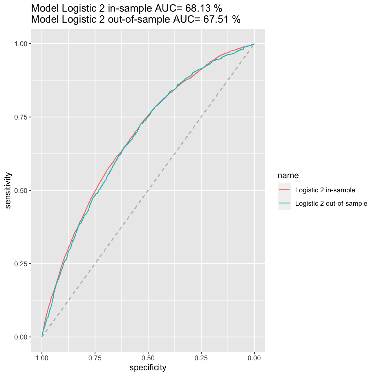
There is a very weak evidence in overfitting, because the ROC curve and AUC statistic has remained roughly the same in both in-sample and out-of-sample cases. Therefore we can assume that overfitting does not occur in our model.
Selecting loans to invest using the model Logistic 2.
Before I look for a better model than logistic 2 let’s see how I can use this model to select loans to invest. Let’s make the simplistic assumption that every loan generates $20 profit if it is paid off and $100 loss if it is charged off for an investor. Let’s use a cut-off value to determine which loans to invest in, that is, if the predicted probability of default for a loan is below this value then I invest in that loan and not if it is above.
To do this I will split the data in three parts: training, validation, and testing.
# splitting the data into training and testing
set.seed(121)
train_test_split <- initial_split(lc_clean, prop = 0.6)
training <- training(train_test_split) #60% of the data is set aside for training
remaining <- testing(train_test_split) #40% of the data is set aside for validation & testing
set.seed(121)
train_test_split <- initial_split(remaining, prop = 0.5)
validation<-training(train_test_split) #50% of the remaining data (20% of total data) will be used for validation
testing<-testing(train_test_split) #50% of the remaining data (20% of total data) will be used for testing
Finding cut-off threshold
I will now use the trained model to determine the optimal cut-off threshold based on the validation test.
logistic2_in<-glm(default~I(annual_inc/1000)+term+grade+loan_amnt, family="binomial", training)
summary(logistic2_in)
##
## Call:
## glm(formula = default ~ I(annual_inc/1000) + term + grade + loan_amnt,
## family = "binomial", data = training)
##
## Deviance Residuals:
## Min 1Q Median 3Q Max
## -1.053 -0.607 -0.487 -0.338 3.237
##
## Coefficients:
## Estimate Std. Error z value Pr(>|z|)
## (Intercept) -2.49e+00 6.64e-02 -37.54 <2e-16 ***
## I(annual_inc/1000) -5.70e-03 6.08e-04 -9.38 <2e-16 ***
## term60 5.02e-01 4.59e-02 10.94 <2e-16 ***
## gradeB 7.34e-01 6.89e-02 10.65 <2e-16 ***
## gradeC 1.07e+00 7.08e-02 15.09 <2e-16 ***
## gradeD 1.32e+00 7.48e-02 17.59 <2e-16 ***
## gradeE 1.42e+00 8.74e-02 16.27 <2e-16 ***
## gradeF 1.70e+00 1.11e-01 15.32 <2e-16 ***
## gradeG 1.78e+00 1.72e-01 10.35 <2e-16 ***
## loan_amnt 1.45e-06 3.03e-06 0.48 0.63
## ---
## Signif. codes: 0 '***' 0.001 '**' 0.01 '*' 0.05 '.' 0.1 ' ' 1
##
## (Dispersion parameter for binomial family taken to be 1)
##
## Null deviance: 18591 on 22721 degrees of freedom
## Residual deviance: 17493 on 22712 degrees of freedom
## AIC: 17513
##
## Number of Fisher Scoring iterations: 5p_val<-predict(logistic2_in, validation, type = "response") #predict probability of default on the validation set
#we select the cutoff threshold using the estimated model and the validation set
profit=0
threshold=0
for(i in 1:100) {
threshold[i]=i/400
one_or_zero_search<-ifelse(p_val>threshold[i],"1","0")
p_class_search<-factor(one_or_zero_search,levels=levels(validation$default))
con_search<-confusionMatrix(p_class_search,validation$default,positive="1")
profit[i]=con_search$table[1,1]*20-con_search$table[1,2]*100
}
ggplot(as.data.frame(threshold), aes(x=threshold,y=profit)) + geom_smooth(method = 'loess', se=0) +labs(title="Profit curve with logistic 2 based on validation set, ")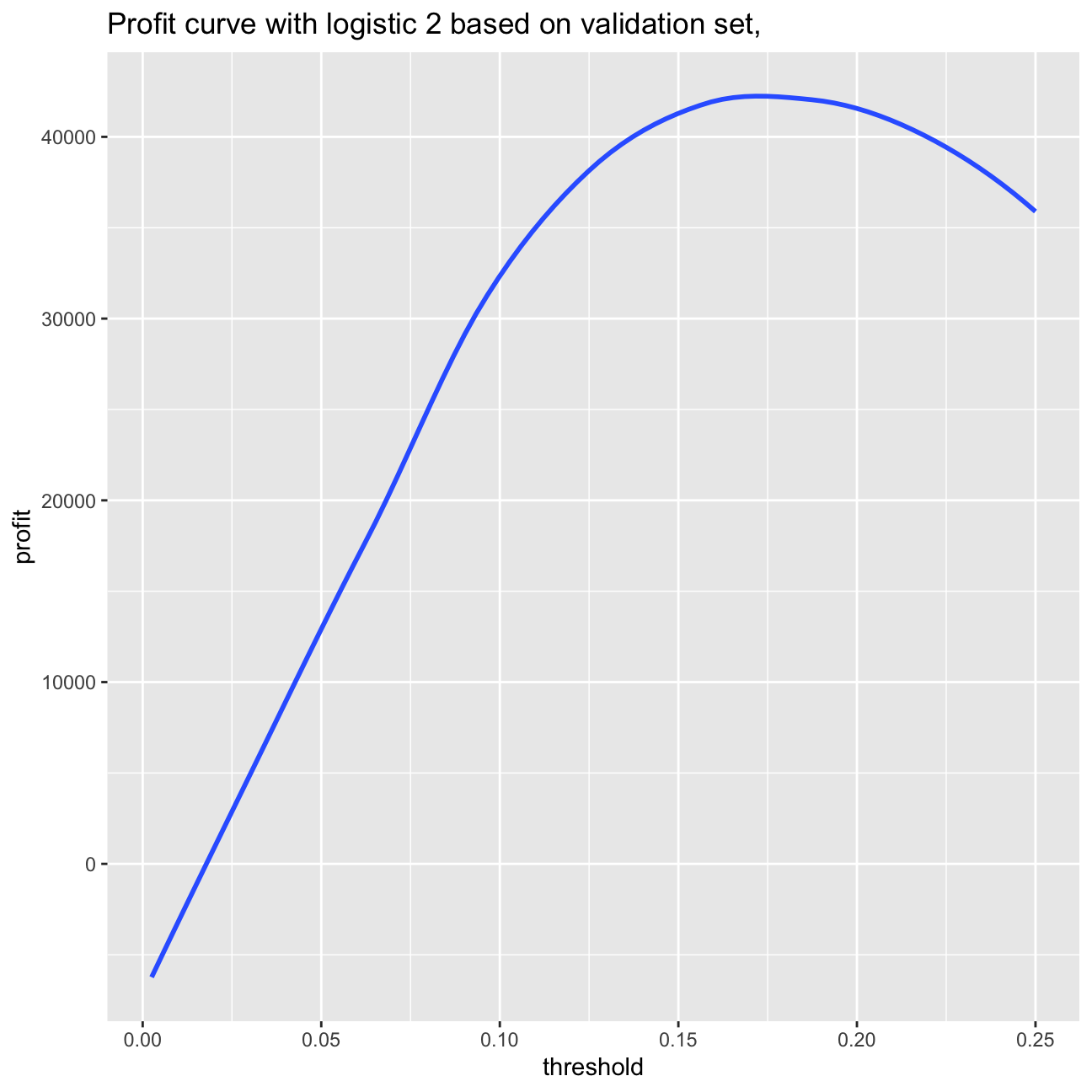
paste0("Based on the validation set: Maximum profit per loan is $", round(max(profit)/nrow(validation),2), " achieved at a threshold of ", threshold[which.is.max(profit)]*100,"%.")## [1] "Based on the validation set: Maximum profit per loan is $5.55 achieved at a threshold of 17%."#calculate probability of default out of sample
p_out<-predict(logistic2_in, testing, type = "response")
#we select the cutoff threshold using the estimated model and the testing set
profitt=0
thresholdt=0
for(i in 1:100) {
thresholdt[i]=i/400
one_or_zero_search_t<-ifelse(p_out>thresholdt[i],"1","0")
p_class_search_t<-factor(one_or_zero_search_t,levels=levels(testing$default))
con_search_t<-confusionMatrix(p_class_search_t,testing$default,positive="1")
profitt[i]=con_search_t$table[1,1]*20-con_search_t$table[1,2]*100
}
ggplot(as.data.frame(thresholdt), aes(x=thresholdt,y=profitt)) + geom_smooth(method = 'loess', se=0) +labs(title="Profit curve with logistic 2 based on testing set, ")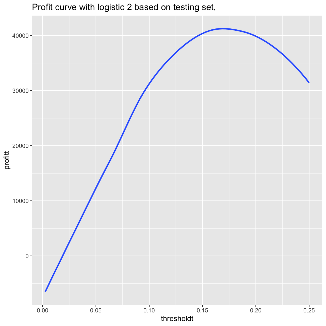
paste0("Based on the testing set: Maximum profit per loan is $", round(max(profitt)/nrow(testing),2), " achieved at a threshold of ", thresholdt[which.is.max(profitt)]*100,"%.")## [1] "Based on the testing set: Maximum profit per loan is $5.62 achieved at a threshold of 17.75%."Based on the validation set, we can observe that the maximum profit per loan is
>’$’5.55
achieved at a threshold of 17% optimal cutoff. In case of using the testing set, I obtain also the cutoff point of 17.5%, however the maximum profit per loan amount to $5.62.
More realistic revenue model
I will now build a more realistic profit and loss model. Each loan has different terms (e.g., different interest rate and different duration) and therefore a different return if fully paid. For example, a 36 month loan of $5000 with installment of $163 per month would generate a return of 163*36/5000-1 if there was no default. Let’s assume that it would generate a loss of -60% if there was a default (the loss is not 100% because the loan may not default immediately and/or the lending club may be able to recover part of the loan).
validation2<-validation%>%
  mutate(default1=as.numeric(default)-1,
         return= ifelse (default1==1, -0.6, term_months*installment/loan_amnt-1))

validation2 %>%
summarize(total_return_percent = sum(return)/n()*100)| total_return_percent |
|---|
| 11.5 |
summary(validation2)## int_rate loan_amnt dti delinq_2yrs
## Min. :0.050 Min. : 500 Min. : 0.00 0 :6766
## 1st Qu.:0.090 1st Qu.: 5500 1st Qu.: 8.07 1 : 630
## Median :0.120 Median :10000 Median :13.32 2 : 129
## Mean :0.121 Mean :11284 Mean :13.24 3 : 32
## 3rd Qu.:0.150 3rd Qu.:15000 3rd Qu.:18.51 4 : 9
## Max. :0.240 Max. :35000 Max. :29.99 5 : 4
## (Other): 4
## annual_inc grade emp_length home_ownership
## Min. : 4200 Length:7574 Length:7574 Length:7574
## 1st Qu.: 41000 Class :character Class :character Class :character
## Median : 60000 Mode :character Mode :character Mode :character
## Mean : 69926
## 3rd Qu.: 83000
## Max. :6000000
##
## verification_status issue_d zip_code addr_state
## Length:7574 Min. :2007-07-01 Length:7574 Length:7574
## Class :character 1st Qu.:2010-05-01 Class :character Class :character
## Mode :character Median :2011-02-01 Mode :character Mode :character
## Mean :2010-11-04
## 3rd Qu.:2011-08-01
## Max. :2011-12-01
##
## loan_status desc purpose title
## Length:7574 Length:7574 Length:7574 Length:7574
## Class :character Class :character Class :character Class :character
## Mode :character Mode :character Mode :character Mode :character
##
##
##
##
## term default term_months installment emp_title
## 36:5570 0:6490 Min. :36.0 Min. : 16 Length:7574
## 60:2004 1:1084 1st Qu.:36.0 1st Qu.: 170 Class :character
## Median :36.0 Median : 295 Mode :character
## Mean :42.4 Mean : 334
## 3rd Qu.:60.0 3rd Qu.: 451
## Max. :60.0 Max. :1303
##
## default1 return
## Min. :0.000 Min. :-0.600
## 1st Qu.:0.000 1st Qu.: 0.120
## Median :0.000 Median : 0.183
## Mean :0.143 Mean : 0.115
## 3rd Qu.:0.000 3rd Qu.: 0.254
## Max. :1.000 Max. : 0.723
## According to the assumption above, I reach a return of 11.45%.
Unfortunately, I cannot use the realized return to select loans to invest (as at the time we make the investment decision we do not know which loan will default). Instead, I can calculate an expected return using the estimated probabilities of default – expected return = return if not default * (1-prob(default)) + return if default * prob(default).
Expected return of the loans
In the nest step, I will calculate the expected return of the loans in the validation set using the logistic 2 model trained in the training set. I will check how the realized return varies as I change \(n\).
expected_return <- p_val*(-0.6)+(1-p_val)*(validation2$term_months*validation2$installment/validation2$loan_amnt-1)

expected_return <-as.data.frame(expected_return) %>%
  arrange(-expected_return)

expected_return_800<-expected_return %>% head(800)

expected_return_800%>%
summarize(expected_return_in_percent = sum(expected_return)/800*100)| expected_return_in_percent |
|---|
| 23.6 |
expected_return_1500<-expected_return %>% head(1500)

expected_return_1500%>%
summarize(expected_return_in_percent =sum(expected_return)/1500*100)| expected_return_in_percent |
|---|
| 20.5 |
expected_return_8000<-expected_return %>% head(8000)

expected_return_8000%>%
summarize(expected_return_in_percent =sum(expected_return)/8000*100)| expected_return_in_percent |
|---|
| 11 |
expected_return_80<-expected_return %>% head(80)

expected_return_80%>%
summarize(expected_return_in_percent =sum(expected_return)/80*100)| expected_return_in_percent |
|---|
| 35.2 |
In case n=800, our expected return amount to 23.64%. In case of increasing n, the perctange value of expected return decreases. If we decrease \(n\), then the expected return in percent increases. We can use the expected return metric as one of the means to select a portfolio, however we should not rely only on this measure. The less loans we choose, the less nominal profit we will obtain. Therefore, it would be smart to use other measures to complement this approach.
For \(n=800\), I will check how sensitive is my answer to the assumption that if a loan defaults I lose 60% of the value.
To answer this question I will assess how the realized return of the 800 loans chosen in my portfolio change if the loss proportion varies from 20%-80%.
expected_return20 <- p_val*(-0.2)+(1-p_val)*(validation2$term_months*validation2$installment/validation2$loan_amnt-1)

expected_return20 <-as.data.frame(expected_return20) %>%
  arrange(-expected_return20)

expected_return_800_20<-expected_return20 %>% head(800)

expected_return_800_20%>%
summarize(sum(expected_return20)/800*100)| sum(expected_return20)/800 * 100 |
|---|
| 33.4 |
expected_return80 <- p_val*(-0.8)+(1-p_val)*(validation2$term_months*validation2$installment/validation2$loan_amnt-1)

expected_return80 <-as.data.frame(expected_return80) %>%
  arrange(-expected_return80)

expected_return_800_80<-expected_return80 %>% head(800)

expected_return_800_80%>%
summarize(sum(expected_return80)/800*100)| sum(expected_return80)/800 * 100 |
|---|
| 19.4 |
expected_return40 <- p_val*(-0.4)+(1-p_val)*(validation2$term_months*validation2$installment/validation2$loan_amnt-1)

expected_return40 <-as.data.frame(expected_return40) %>%
  arrange(-expected_return40)

expected_return_800_40<-expected_return40 %>% head(800)

expected_return_800_40%>%
summarize(sum(expected_return40)/800*100)| sum(expected_return40)/800 * 100 |
|---|
| 28.3 |
If we lose 20% on default loans, we have expected return on the 800 loans as 33.36%. If we lose 80% on default loans, we have expected return on the 800 loans as 19.44%. The return changes but we still gain profit from it. The expected return increases more if the loss is small. It means that our answer is not this much sensitive to the assupmtion that if the loan defaults, we lose 60% of the value.
Models experimentation
I will now experiment with different models using more features, interactions, and non-linear transformations.
I will include below only my best model and explain why I chose it.
#showing best model
#splitting the data again
set.seed(121)
train_test_split <- initial_split(lc_clean, prop = 0.6)
training <- training(train_test_split) #60% of the data is set aside for training
remaining <- testing(train_test_split)

train_test_split <- initial_split(remaining, prop = 0.5)
validation<-training(train_test_split)
testing<-testing(train_test_split)

logistic_wild<-glm(default~
                     poly(I(annual_inc/1000),3)+
                     term+
                     grade+
                     poly(int_rate,3):loan_amnt+
                     issue_d*grade, family="binomial", training)
summary(logistic_wild)
##
## Call:
## glm(formula = default ~ poly(I(annual_inc/1000), 3) + term +
## grade + poly(int_rate, 3):loan_amnt + issue_d * grade, family = "binomial",
## data = training)
##
## Deviance Residuals:
## Min 1Q Median 3Q Max
## -1.211 -0.606 -0.476 -0.320 3.000
##
## Coefficients:
## Estimate Std. Error z value Pr(>|z|)
## (Intercept) -1.22e+01 2.89e+00 -4.23 2.3e-05 ***
## poly(I(annual_inc/1000), 3)1 -1.49e+02 4.00e+01 -3.72 0.00020 ***
## poly(I(annual_inc/1000), 3)2 -1.88e+02 7.05e+01 -2.66 0.00773 **
## poly(I(annual_inc/1000), 3)3 -1.18e+02 2.87e+01 -4.12 3.8e-05 ***
## term60 5.02e-01 4.91e-02 10.21 < 2e-16 ***
## gradeB 1.33e+01 3.35e+00 3.97 7.2e-05 ***
## gradeC 1.31e+01 3.36e+00 3.89 9.9e-05 ***
## gradeD 1.03e+01 3.57e+00 2.87 0.00409 **
## gradeE 7.04e+00 4.38e+00 1.61 0.10845
## gradeF 1.57e+01 6.26e+00 2.51 0.01212 *
## gradeG 3.05e+01 1.02e+01 2.98 0.00290 **
## issue_d 6.40e-04 1.93e-04 3.31 0.00092 ***
## poly(int_rate, 3)1:loan_amnt 2.78e-03 4.71e-04 5.91 3.3e-09 ***
## poly(int_rate, 3)2:loan_amnt -1.99e-03 4.46e-04 -4.45 8.6e-06 ***
## poly(int_rate, 3)3:loan_amnt 1.10e-03 2.87e-04 3.82 0.00013 ***
## gradeB:issue_d -8.65e-04 2.25e-04 -3.85 0.00012 ***
## gradeC:issue_d -8.32e-04 2.26e-04 -3.69 0.00022 ***
## gradeD:issue_d -6.25e-04 2.40e-04 -2.61 0.00905 **
## gradeE:issue_d -4.04e-04 2.94e-04 -1.38 0.16879
## gradeF:issue_d -9.67e-04 4.19e-04 -2.31 0.02103 *
## gradeG:issue_d -1.96e-03 6.87e-04 -2.85 0.00432 **
## ---
## Signif. codes: 0 '***' 0.001 '**' 0.01 '*' 0.05 '.' 0.1 ' ' 1
##
## (Dispersion parameter for binomial family taken to be 1)
##
## Null deviance: 18591 on 22721 degrees of freedom
## Residual deviance: 17378 on 22701 degrees of freedom
## AIC: 17420
##
## Number of Fisher Scoring iterations: 10#calculate probability of default in the training sample
p_wild_in<-predict(logistic_wild, training, type = "response")
#ROC curve using in-sample predictions
ROC_logistic_wild <- roc(training$default,p_wild_in)
#AUC using in-sample predictions
AUC_logistic_wild<-round(auc(training$default,p_wild_in)*100, digits=2)
#quick check for overfitting
#calculate probability of default out of sample
p_wild_out<-predict(logistic_wild, testing, type = "response")
#ROC curve using out-of-sample predictions
ROC_logistic_wild_out <- roc(testing$default,p_wild_out)
#AUC using out-of-sample predictions
AUC_logistic_wild_out <- round(auc(testing$default,p_wild_out)*100, digits=2)
#plot in the same figure both ROC curves and print the AUC of both curves in the title
ggroc(list("Logistic Wild in-sample"=ROC_logistic_wild, "Logistic Wild out-of-sample"=ROC_logistic_wild_out))+ggtitle(paste("Model Logistic Wild in-sample AUC=",round(auc(training$default,p_wild_in)*100, digits=2),"%\nModel Logistic Wild out-of-sample AUC=",round(auc(testing$default,p_wild_out)*100, digits=2),"%")) +
geom_segment(aes(x = 1, xend = 0, y = 0, yend = 1), color="grey", linetype="dashed")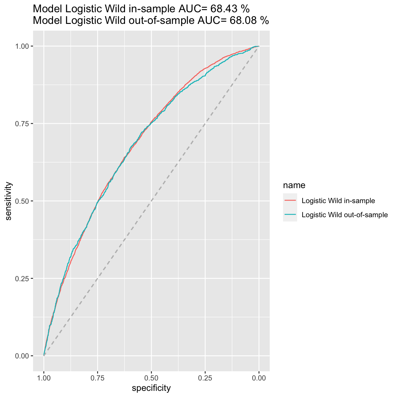
#very weak evidence of overfitting, we can compare now our model logistic_wild to logistic2

logistic2_in<-glm(default~I(annual_inc/1000)+term+grade+loan_amnt, family="binomial", training)

#calculate probability of default in the training sample of model logistic2_in
p_in<-predict(logistic2_in, training, type = "response")

#ROC curve using in-sample predictions
ROC_logistic2_in <- roc(training$default,p_in)
#AUC using in-sample predictions
AUC_logistic2_in<-round(auc(training$default,p_in)*100, digits=2)
#plot in the same figure both ROC curves and print the AUC of both curves in the title
ggroc(list("Logistic 2"=ROC_logistic2_in, "Logistic Wild"=ROC_logistic_wild))+ggtitle(paste("Model Logistic 2 on training set AUC=",round(auc(training$default,p_in)*100, digits=2),"%\nModel Logistic Wild on training set AUC=",round(auc(training$default,p_wild_in)*100, digits=2),"%"))    +
geom_segment(aes(x = 1, xend = 0, y = 0, yend = 1), color="grey", linetype="dashed")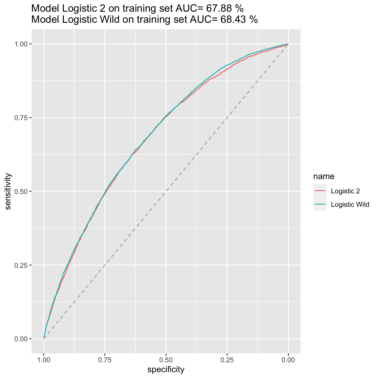
#calculate probability of default in the training sample
p_wild_val<-predict(logistic_wild, validation, type = "response")
expected_return60l <- p_wild_val*(-0.6)+(1-p_wild_val)*(validation$term_months*validation$installment/validation$loan_amnt-1)

expected_return60l <-as.data.frame(expected_return60l) %>%
  arrange(-expected_return60l)

expected_return_800_60l<-expected_return60l %>% head(800)

expected_return_800_60l%>%
summarize(expected_return_in_percent= sum(expected_return60l)/800*100)| expected_return_in_percent |
|---|
| 24.3 |
p_val<-predict(logistic2_in, validation, type = "response")
expected_return <- p_val*(-0.6)+(1-p_val)*(validation$term_months*validation$installment/validation$loan_amnt-1)

expected_return <-as.data.frame(expected_return) %>%
  arrange(-expected_return)

expected_return_800<-expected_return %>% head(800)

expected_return_800%>%
summarize(expected_return_in_percent = sum(expected_return)/800*100)| expected_return_in_percent |
|---|
| 23.7 |
My best model is model logistic_wild. I managed to achieve the AIC at the level of 17420 and AUC of the model accounting to 68,43%.When it comes to expected returns, the ones based on model logistic_wild bring return amounting to 24,34% (in comparison to 23,70% from model logistic2) basing it on the validation set. When searching the model, I tried the LASSO method on training split, I tried as well to add variables on inflation and price, however, they would increase my AIC and decrease the AUC. Therefore, I sticked to model logistic_wild.
Predicting outcomes for the testing data
The file “Assessment Data_2020.csv” contains information on almost 1800 new loans. I will use my best model form the previous point to choose 200 loans to invest. For this I will assume that the loss proportion is 60%.
lc_assessment<- read_csv("~/Documents/LBS/Data Science/Session 05/Assessment Data_2020.csv")
 lc_assessment<-  lc_assessment %>%
   janitor::clean_names() %>% # use janitor::clean_names()
  mutate(
    issue_d = lubridate::mdy(issue_d),  # lubridate::mdy() to fix date format
    term = factor(term_months),     # turn 'term' into a categorical variable
    delinq_2yrs = factor(delinq_2yrs)) # turn 'delinq_2yrs' into a categorical variable

#  lc_assessment %>% head(10)

 p_assessment<-predict(logistic_wild, lc_assessment, type = "response")

  p_assessment %>% head(10)
## 1 2 3 4 5 6 7 8 9 10
## 0.0873 0.1225 0.0498 0.1685 0.2225 0.1730 0.1021 0.0771 0.1113 0.1775 expected_return_assessment <- p_assessment*(-0.6)+(1-p_assessment)*(lc_assessment$term_months*lc_assessment$installment/lc_assessment$loan_amnt-1)
lc_assessment_total<- lc_assessment %>%
mutate(expected_return=expected_return_assessment ) %>%
arrange(-expected_return )
lc_assessment_total_200 <- lc_assessment_total %>%
head(200) %>%
mutate( agnieszka_prawda= 1)
merged_assessment<- merge(x = lc_assessment_total, y = lc_assessment_total_200, by = "loan_number", all.x = TRUE) %>%
select(loan_number, agnieszka_prawda)
merged_assessment<- replace_na(merged_assessment,list(agnieszka_prawda=0))
merged_assessment %>% head(20) #glimpse for 10 rows| loan_number | agnieszka_prawda |
|---|---|
| 1 | 0 |
| 2 | 0 |
| 3 | 0 |
| 4 | 0 |
| 5 | 1 |
| 6 | 0 |
| 7 | 0 |
| 8 | 0 |
| 9 | 0 |
| 10 | 0 |
| 11 | 0 |
| 12 | 0 |
| 13 | 0 |
| 14 | 0 |
| 15 | 1 |
| 16 | 0 |
| 17 | 0 |
| 18 | 0 |
| 19 | 0 |
| 20 | 1 |
Critique
No data science engagement is perfect. Therefore, I decided to include a critique of my project in here to reflect on the limitations of the analysis and ways for future improvement.
First of all, I believe collecting some more historical data on all the loan takers, on how they coped with their liabilities and credit history. I tried to use models on inflation and on bond prices however, the data did not improve my model, so I decided to drop it. Before using it in practice, I would like to try and find true value of the return in case of default instead of 60% assumed. I would also try to run Rigde regression and see how is compares to LASSO ( the best model in the homework).
Data on gender or race
We do not include data on race or gender as our model could become bias and disciminate poeple of particular sex or skin color. Even if such variables may be good predictors, they may sometimes be not the best choice for machine learning if not carefully trained and considered. It is an aesthetic approach to data and modelling. We need to remember that when using machine learning methods, the models may sometimes take spourious values as significant ones and become sexist or racist.
