Predicting Prices for Munich Airbnb
Airbnb is a prime example of a disruptive innovation, that is now one of the largest marketplaces for accomodation with over 7 million properties in more than 220 countries. With this project I sought to utilize scraped data from Airbnb listings to carry out statistical analyses and ultimately predict the total cost for two people staying four nights in the city of Munich, Germany.
After initial cleaning and wrangling of the dataset, I carried out an exploratory data analysis (EDA) to investigate existing relationships between variables, especially within and between price, neighbourhood / region, room and property type, as well as reviews and cancellation policy. As I will explain in greater detail below, I grouped the neighbourhoods within zones based on both personal experience and an official map of zones based on accomodation quality and price from the city of Munich. Key observations within our EDA were that there is a heavily right skewed distribution of price and reviews, and that no linear relationship regarding price could be observed; this led us to use the log of the total price for 4 days going forward with our regression.
I progressively improved the model of regression by investigating the effect of all variables as displayed through t- and p-values. My final and best model includes the most extensive list of variables, including for example the addition of logical variables for the only two significant amenities (elevator and shampoo). I ultimately arrived at an adjusted R-squared value of around 40%. Given that the correlation matrix and other early analyses showed rather weak / limited relationships between variables, I believe this is a good result based on the given dataset. Lastly, plots of residuals (i.e. QQ-plot, residuals vs. fitted) as well as variation inflation factor analyses showed that all assumptions of a linear regression (L-I-N-E) were met.
listings <- vroom("http://data.insideairbnb.com/germany/bv/munich/2020-06-20/data/listings.csv.gz") %>%
    clean_names()
#glimpse(listings) # checking variable headers
Data Preprocessing
Selecting variables and changing to the relevant type
I first select all potentially relevant variables from my data frame. The data is cleaned into number or factor to begin Exploratory Data Analysis (EDA). The raw dataset I create here is called munich_listings.
#Selecting all the relevant variables
munich_listings<- listings %>%
  select(id,
         host_is_superhost,
         host_listings_count,
         neighbourhood_cleansed,
         latitude,
         longitude,
         property_type,
         room_type,
         accommodates,
         bathrooms,
         bedrooms,
         beds,
         bed_type,
          #square_feet, we noticed that a lot of values are missing so excluded this variable
         price,
         security_deposit,
         cleaning_fee,
         guests_included,
         extra_people,
         minimum_nights,
         maximum_nights,
         number_of_reviews,
         reviews_per_month,
         review_scores_rating,
         review_scores_accuracy,
         review_scores_cleanliness,
         review_scores_checkin,
         review_scores_communication,
         review_scores_location,
         review_scores_value,
         is_location_exact,
         amenities,
         instant_bookable,
         cancellation_policy,
         availability_365,
         availability_90,
         last_review,
         listing_url,
         last_scraped) %>%
#Converting characters to "doubles" and factors where appropriate
  mutate(neighbourhood_cleansed=factor(neighbourhood_cleansed),
         property_type,
         room_type=factor(room_type),
         price=parse_number(price),
         security_deposit=parse_number(security_deposit),
         cleaning_fee=parse_number(cleaning_fee),
         extra_people=parse_number(extra_people),
         cancellation_policy=factor(cancellation_policy),
         bed_type=factor(bed_type),
         amenities_count= str_count(listings$amenities, ","))
#Inspecting data frame to make sure all the variables are correctly attributed
glimpse(munich_listings) ## Rows: 11,172
## Columns: 39
## $ id <dbl> 36720, 97945, 114695, 127383, 157808, 159…
## $ host_is_superhost <lgl> FALSE, TRUE, TRUE, TRUE, FALSE, FALSE, TR…
## $ host_listings_count <dbl> 1, 1, 3, 2, 0, 1, 1, 1, 2, 1, 1, 1, 2, 2,…
## $ neighbourhood_cleansed <fct> Ludwigsvorstadt-Isarvorstadt, Hadern, Ber…
## $ latitude <dbl> 48.1, 48.1, 48.1, 48.2, 48.2, 48.1, 48.1,…
## $ longitude <dbl> 11.6, 11.5, 11.6, 11.6, 11.6, 11.5, 11.5,…
## $ property_type <chr> "Apartment", "Apartment", "Apartment", "A…
## $ room_type <fct> Entire home/apt, Entire home/apt, Entire …
## $ accommodates <dbl> 2, 2, 5, 4, 2, 3, 4, 2, 2, 2, 2, 1, 16, 5…
## $ bathrooms <dbl> 1.0, 1.0, 1.0, 1.0, 1.0, 1.0, 1.0, 1.0, 1…
## $ bedrooms <dbl> 1, 1, 1, 1, 1, 1, 1, 1, 1, 1, 1, 1, 1, 1,…
## $ beds <dbl> 1, 1, 3, 1, 1, 1, 2, 1, 1, 0, 1, 1, 0, 3,…
## $ bed_type <fct> Futon, Real Bed, Real Bed, Real Bed, Real…
## $ price <dbl> 95, 80, 95, 120, 35, 55, 55, 65, 54, 67, …
## $ security_deposit <dbl> 100, NA, 500, NA, 100, 0, 200, NA, 190, N…
## $ cleaning_fee <dbl> 30, 10, 60, 28, 10, 60, 20, NA, 32, NA, 0…
## $ guests_included <dbl> 1, 1, 1, 1, 1, 1, 2, 1, 2, 1, 2, 1, 1, 1,…
## $ extra_people <dbl> 30, 10, 50, 0, 15, 30, 15, 0, 0, 0, 0, 20…
## $ minimum_nights <dbl> 2, 2, 2, 2, 1, 3, 2, 3, 1, 2, 3, 2, 1, 1,…
## $ maximum_nights <dbl> 730, 90, 30, 14, 36, 90, 1125, 14, 4, 30,…
## $ number_of_reviews <dbl> 25, 131, 53, 84, 0, 33, 467, 64, 211, 89,…
## $ reviews_per_month <dbl> 0.34, 1.23, 0.49, 0.76, NA, 0.31, 4.39, 0…
## $ review_scores_rating <dbl> 98, 97, 95, 98, NA, 93, 99, 91, 97, 97, 9…
## $ review_scores_accuracy <dbl> 10, 10, 9, 10, NA, 9, 10, 9, 10, 10, 10, …
## $ review_scores_cleanliness <dbl> 10, 10, 10, 10, NA, 9, 10, 9, 10, 10, 9, …
## $ review_scores_checkin <dbl> 10, 10, 10, 10, NA, 9, 10, 10, 10, 10, 10…
## $ review_scores_communication <dbl> 10, 10, 10, 10, NA, 10, 10, 10, 10, 10, 1…
## $ review_scores_location <dbl> 10, 9, 9, 10, NA, 9, 10, 9, 10, 10, 10, 1…
## $ review_scores_value <dbl> 9, 9, 9, 10, NA, 9, 10, 9, 9, 10, 9, 10, …
## $ is_location_exact <lgl> TRUE, TRUE, TRUE, TRUE, TRUE, TRUE, TRUE,…
## $ amenities <chr> "{TV,\"Cable TV\",Internet,Wifi,Kitchen,H…
## $ instant_bookable <lgl> FALSE, FALSE, FALSE, FALSE, FALSE, TRUE, …
## $ cancellation_policy <fct> strict_14_with_grace_period, flexible, st…
## $ availability_365 <dbl> 0, 82, 59, 6, 0, 142, 260, 90, 0, 111, 1,…
## $ availability_90 <dbl> 0, 2, 48, 6, 0, 4, 46, 90, 0, 43, 0, 89, …
## $ last_review <date> 2017-07-22, 2019-10-03, 2019-10-06, 2020…
## $ listing_url <chr> "https://www.airbnb.com/rooms/36720", "ht…
## $ last_scraped <date> 2020-06-21, 2020-06-20, 2020-06-21, 2020…
## $ amenities_count <int> 10, 35, 36, 37, 24, 37, 32, 19, 31, 22, 2…In munich_listings, we have 11172 items and 46 columns.
- neighbourhood_cleansed, room_type, cancellation_policy and bed_type are changed into factors.
- price, security_deposit, cleaning_fee, extra_people and amenities_count are changed into numbers.
- host_is_superhost,
- is_location_exact,
-
instant_bookable
as logical variables - neighbourhood_cleansed,
- room_type,
- bed_type,
-
cancellation_policy
as factor variables - amenities,
-
property_type
as character variables
Data cleaning
I now create a new data frame called munich_listings_cleaned to do some required changes. Here, I deal with missing values/NAs, and clean the data for property type. Also, I filter the items upon min/max nights and accommodates for the 2 people to live for 4 nights.
Filter dataset for two people and 4 nights
#Clean dataset for cleaning_fee, security_deposit, property_type, minimum_nights and accommodates
munich_listings_cleaned <- munich_listings %>%
  mutate(cleaning_fee = case_when(      #considering cleaning_fee as 0 if displayed as NA
    is.na(cleaning_fee) ~ 0,
    TRUE ~ cleaning_fee),
    security_deposit = case_when(      #considering security_deposit as 0 if displayed as NA
    is.na(security_deposit) ~ 0,
    TRUE ~ security_deposit),
    prop_type_simplified = case_when(   #regrouping of property_types: put all less popular property types into "Other"
    property_type %in% c("Apartment",
                         "House",
                         "Condominium",
                         "Loft")~ property_type ,
    TRUE ~ "Other"),
    prop_type_simplified=factor(prop_type_simplified)) %>% #creating factors
  filter(minimum_nights<=4,
         maximum_nights>=4,
         accommodates>=2) #filtering dataframe for 2 people and 4 nights
#Visually inspecting cleaned data set
#glimpse(munich_listings_cleaned)
#skim(munich_listings_cleaned)For the NAs: I assume NA as 0 in cleaning fee and security deposit, which means I can book Airbnb without paying for these 2 services. So I didn’t make deletion here.
For property_type: I arranged the data set and find the top 5 kinds of Airbnbs in Munich, which are Apartment, House, Condominium, Loft and others. I transferred the variable into factors.
Filtering: I filter the room with minimum_night and maximum_night so that they can be booked for a 4-night stay. Also, the room should accommodate at least 2 people.
Calculating total price
Then, I construct the formula for the total price of 4 days into data frame munich_listings_total_price:
I create total_price_4_days as my target variable for regression representing total price of 4-night stay of two people. The if_else statement will allow to include the option of adding 1 extra guest to an AirBnB that has accommodates = 1. The final multiplier of 1.142 is the 14.2% service fee for AirBnB bookings that the company charges per booking.
munich_listings_total_price<-munich_listings_cleaned %>%
  mutate(total_price_4_days=price*4+ #calculating the total price for 4 days 2 guests
           cleaning_fee+
           if_else(guests_included==1,
                   extra_people*4,0))
Creating a new data frame for further analysis
I will now create a new data frame called “munich_listings_region” grouping the Airbnbs geographically and making some changes for the subsequent analysis.
Three variable classes are created:- region: grouped into 5 by the average price of each neighborhood
- rating_group: grouped into 3 by whether the rating is over 90
- Amenities: numerous different amenity words were checked for significance, only two remained. Interestingly they are shampoo and elevator.
munich_listings_region <- munich_listings_total_price %>%
  mutate(
region = case_when( #creating variable that clusters neighbourhoods for further analysis
      neighbourhood_cleansed=="Altstadt-Lehel"~"zone_1",
      neighbourhood_cleansed=="Ludwigsvorstadt-Isarvorstadt"~"zone_1",
      neighbourhood_cleansed=="Maxvorstadt"~"zone_1",
      neighbourhood_cleansed=="Schwabing-West"~"zone_2",
      neighbourhood_cleansed=="Au-Haidhausen"~"zone_2",
      neighbourhood_cleansed=="Sendling"~"zone_2",
      neighbourhood_cleansed=="Sendling-Westpark"~"zone_2",
      neighbourhood_cleansed=="Schwanthalerhöhe"~"zone_1",
      neighbourhood_cleansed=="Neuhausen-Nymphenburg"~"zone_3",
      neighbourhood_cleansed=="Moosach"~"zone_5",
      neighbourhood_cleansed=="Milbertshofen-Am Hart"~"zone_5",
      neighbourhood_cleansed=="Schwabing-Freimann"~"zone_3",
      neighbourhood_cleansed=="Bogenhausen"~"zone_4",
      neighbourhood_cleansed=="Berg am Laim"~"zone_4",
      neighbourhood_cleansed=="Tudering-Riem"~"zone_1",
      neighbourhood_cleansed=="Ramersdorf-Perlach"~"zone_5",
      neighbourhood_cleansed=="Obergiesing"~"zone_2",
      neighbourhood_cleansed=="Untergiesing-Harlaching"~"zone_4",
      neighbourhood_cleansed=="Thalkirchen-Obersendling-Forstenried-Fürstenried-Solln"~"zone_3",
      neighbourhood_cleansed=="Hadern"~"zone_5",
      neighbourhood_cleansed=="Pasing-Obermenzing"~"zone_3",
      neighbourhood_cleansed=="Aubing-Lochhausen-Langwied"~"zone_4",
      neighbourhood_cleansed=="Allach-Untermenzing"~"zone_3",
      neighbourhood_cleansed=="Feldmoching-Hasenbergl"~"zone_3",
      neighbourhood_cleansed=="Laim"~"zone_5"
      ),
rating_group= case_when( #clustering review_scores_rating to 2 groups
  review_scores_rating <90 ~ "Under 90",
  TRUE ~ "Over 90"),
# is_pool=case_when(
#   grepl("Pool", amenities, fixed=TRUE) ~ TRUE,
#   TRUE ~FALSE),
# is_gym=case_when(
#   grepl("Gym", amenities, fixed=TRUE) ~ TRUE,
#   TRUE ~FALSE),
# is_private_entrance=case_when(
#   grepl("Private entrance", amenities, fixed=TRUE) ~ TRUE,
#   TRUE ~FALSE),
# is_balcony=case_when(
#   grepl("balcony", amenities, fixed=TRUE) ~ TRUE,
#   TRUE ~FALSE),
# is_kitchen=case_when(
#   grepl("Kitchen", amenities, fixed=TRUE) ~ TRUE,
#   TRUE ~FALSE),
is_elevator=case_when( # turned out to be significant
  grepl("Elevator",
        amenities,
        fixed=TRUE) ~ TRUE,
  TRUE ~FALSE),
# is_washer=case_when(
#   grepl("Washer", amenities, fixed=TRUE) ~ TRUE,
#   TRUE ~FALSE),
# is_dryer=case_when(
#   grepl("Dryer", amenities, fixed=TRUE) ~ TRUE,
#   TRUE ~FALSE),
# is_free_parking=case_when(
#   grepl("Free parking on premises", amenities, fixed=TRUE) ~ TRUE,
#   TRUE ~FALSE),
# is_paid_parking=case_when(
#   grepl("Paid parking off premises", amenities, fixed=TRUE) ~ TRUE,
#   TRUE ~FALSE),
# is_essentials=case_when(
#   grepl("Essentials", amenities, fixed=TRUE) ~ TRUE,
#   TRUE ~FALSE),
is_shampoo=case_when( #turned out to be significant
  grepl("Shampoo",
        amenities,
        fixed=TRUE) ~ TRUE,
  TRUE ~FALSE))
# is_host_greets_you=case_when(
#   grepl("Host greets you", amenities, fixed=TRUE) ~ TRUE,
#   TRUE ~FALSE),
# is_garden=case_when(
#   grepl("Garden or backyard", amenities, fixed=TRUE) ~ TRUE,
#   TRUE ~FALSE))


munich_listings_region <- munich_listings_region %>%  #cleaning dataframe from all the missing values
 na.omit()
Key variable descriptions
Here are description of the key variables in our dataset:-
dependent variable:
-
total_price_4_days
-
independent variable:
-
property_type: type of accommodation (House, Apartment, etc.) -
room_type: - Entire home/apt (guests have entire place to themselves)
- Private room (Guests have private room to sleep, all other rooms shared)
- Shared room (Guests sleep in room shared with others)
-
number_of_reviews: Total number of reviews for the listing -
review_scores_rating: Average review score (0 - 100) -
longitude , latitude: geographical coordinates to help us locate the listing -
region: factor. Region the Airbnb is at grouping by house price. factored 1-5 from high price to low price -
prop_type_simplified: type of accommodation (House, Apartment, Loft, Condominium) -
room_type:Entire home/apt, Private room, Shared room -
number_of_reviews: Total number of reviews for the listing -
reviews_per_month: Number of reviews per month -
review_scores_: Rating for in reviews in different aspects -
rating_group: Average review score (0 - 100) grouped by 90 -
longitude , latitude: geographical coordinates to help us locate the listing -
region: factor. Region the Airbnb is at grouping by house price. factored 1-5 from high price to low price -
availability_365: Available days in the last 365 days -
is_elevatorandis_shampoo: Whether there is elevator or shampoo facilitated
Exploratory Data Analysis
Now that I have cleaned my data sets for the specific target (4 nights, 2 people), I will conduct an exploratory data analysis.
Summary statistics and favstats
#summary to check for NA's and general statistics
#summary(munich_listings_region)

#running favstats on some interesting variable combinations and keeping the most interesting ones
favstats(price~accommodates, data=munich_listings_region) | accommodates | min | Q1 | median | Q3 | max | mean | sd | n | missing |
|---|---|---|---|---|---|---|---|---|---|
| 2 | 15 | 50 | 70 | 100 | 999 | 85.5 | 65.1 | 3648 | 0 |
| 3 | 12 | 64 | 90 | 135 | 1e+03 | 111 | 79.9 | 893 | 0 |
| 4 | 11 | 80 | 115 | 180 | 8e+03 | 154 | 288 | 1163 | 0 |
| 5 | 35 | 94 | 139 | 200 | 1.12e+03 | 181 | 146 | 205 | 0 |
| 6 | 32 | 96.2 | 172 | 300 | 1e+03 | 234 | 199 | 214 | 0 |
| 7 | 34 | 89 | 140 | 215 | 700 | 181 | 131 | 44 | 0 |
| 8 | 25 | 128 | 228 | 414 | 995 | 308 | 251 | 66 | 0 |
| 9 | 65 | 125 | 226 | 288 | 950 | 311 | 325 | 6 | 0 |
| 10 | 25 | 196 | 294 | 612 | 1.45e+03 | 437 | 375 | 18 | 0 |
| 11 | 149 | 262 | 475 | 2.74e+03 | 9e+03 | 2.52e+03 | 4.32e+03 | 4 | 0 |
| 12 | 125 | 285 | 325 | 551 | 800 | 409 | 221 | 10 | 0 |
| 13 | 39 | 39 | 39 | 39 | 39 | 39 | 1 | 0 | |
| 14 | 185 | 242 | 300 | 360 | 420 | 302 | 118 | 3 | 0 |
| 16 | 35 | 35 | 35 | 111 | 839 | 145 | 250 | 10 | 0 |
favstats(price~neighbourhood_cleansed, data=munich_listings_region)| neighbourhood_cleansed | min | Q1 | median | Q3 | max | mean | sd | n | missing |
|---|---|---|---|---|---|---|---|---|---|
| Allach-Untermenzing | 18 | 42 | 75 | 110 | 530 | 111 | 113 | 35 | 0 |
| Altstadt-Lehel | 25 | 80 | 120 | 180 | 800 | 153 | 111 | 222 | 0 |
| Au-Haidhausen | 25 | 60 | 85 | 120 | 1.45e+03 | 115 | 116 | 408 | 0 |
| Aubing-Lochhausen-Langwied | 16 | 41.5 | 65 | 149 | 380 | 99 | 81.3 | 56 | 0 |
| Berg am Laim | 25 | 55 | 76.5 | 131 | 400 | 103 | 75.7 | 110 | 0 |
| Bogenhausen | 23 | 57 | 80 | 120 | 500 | 97.9 | 66.4 | 297 | 0 |
| Feldmoching-Hasenbergl | 25 | 45 | 62.5 | 98.2 | 350 | 88.4 | 68 | 74 | 0 |
| Hadern | 15 | 45 | 79 | 100 | 350 | 84.4 | 58.4 | 73 | 0 |
| Laim | 20 | 50 | 80 | 121 | 585 | 100 | 82.8 | 216 | 0 |
| Ludwigsvorstadt-Isarvorstadt | 28 | 70 | 100 | 150 | 9e+03 | 172 | 499 | 717 | 0 |
| Maxvorstadt | 28 | 65 | 90 | 140 | 999 | 122 | 107 | 666 | 0 |
| Milbertshofen-Am Hart | 12 | 49 | 70 | 100 | 400 | 86 | 58.6 | 249 | 0 |
| Moosach | 25 | 50 | 70 | 100 | 800 | 101 | 113 | 103 | 0 |
| Neuhausen-Nymphenburg | 21 | 52.2 | 79.5 | 120 | 899 | 104 | 83.7 | 434 | 0 |
| Obergiesing | 15 | 50 | 80 | 130 | 700 | 109 | 98.9 | 213 | 0 |
| Pasing-Obermenzing | 21 | 46 | 70 | 125 | 800 | 105 | 104 | 119 | 0 |
| Ramersdorf-Perlach | 15 | 45 | 60 | 90 | 420 | 75 | 49.4 | 215 | 0 |
| Schwabing-Freimann | 20 | 55 | 80 | 120 | 1e+03 | 106 | 101 | 339 | 0 |
| Schwabing-West | 11 | 56.2 | 80 | 120 | 1e+03 | 107 | 89.6 | 446 | 0 |
| Schwanthalerhöhe | 25 | 70 | 104 | 160 | 1e+03 | 136 | 115 | 260 | 0 |
| Sendling | 25 | 59.2 | 90 | 135 | 590 | 113 | 88.5 | 258 | 0 |
| Sendling-Westpark | 20 | 52 | 80 | 120 | 990 | 109 | 105 | 208 | 0 |
| Thalkirchen-Obersendling-Forstenried-Fürstenried-Solln | 25 | 50 | 75 | 120 | 1.12e+03 | 98.8 | 93.5 | 211 | 0 |
| Tudering-Riem | 30 | 50 | 75 | 120 | 999 | 127 | 152 | 161 | 0 |
| Untergiesing-Harlaching | 28 | 60 | 80 | 120 | 500 | 107 | 77.7 | 195 | 0 |
favstats(price~host_is_superhost, data=munich_listings_region)| host_is_superhost | min | Q1 | median | Q3 | max | mean | sd | n | missing |
|---|---|---|---|---|---|---|---|---|---|
| FALSE | 11 | 60 | 88 | 130 | 9e+03 | 119 | 206 | 5280 | 0 |
| TRUE | 18 | 50 | 75 | 110 | 1e+03 | 101 | 91.9 | 1005 | 0 |
favstats(price~prop_type_simplified, data=munich_listings_region)| prop_type_simplified | min | Q1 | median | Q3 | max | mean | sd | n | missing |
|---|---|---|---|---|---|---|---|---|---|
| Apartment | 11 | 59 | 85 | 129 | 8e+03 | 113 | 157 | 5510 | 0 |
| Condominium | 19 | 55.2 | 89.5 | 150 | 995 | 139 | 149 | 182 | 0 |
| House | 20 | 45 | 65 | 100 | 890 | 96.7 | 107 | 216 | 0 |
| Loft | 35 | 75 | 99 | 144 | 9e+03 | 236 | 907 | 98 | 0 |
| Other | 20 | 54 | 89 | 144 | 999 | 144 | 184 | 279 | 0 |
favstats(price~minimum_nights, data=munich_listings_region)| minimum_nights | min | Q1 | median | Q3 | max | mean | sd | n | missing |
|---|---|---|---|---|---|---|---|---|---|
| 1 | 15 | 53 | 80 | 125 | 8e+03 | 114 | 197 | 2351 | 0 |
| 2 | 11 | 60 | 85 | 129 | 9e+03 | 116 | 216 | 2649 | 0 |
| 3 | 15 | 60 | 89 | 144 | 1.45e+03 | 126 | 129 | 967 | 0 |
| 4 | 23 | 60 | 90 | 147 | 800 | 116 | 85.8 | 318 | 0 |
Correlation Matrix
From the summary and favstats investigations, I have decided to conduct further exploratory data analysis through ggplot2. I will first build a correlation martix to spot the relationships between the particular variables.
munich_listing_is_numeric<-munich_listings_region[,sapply(munich_listings_region,is.numeric),with=FALSE]%>%
  na.omit() #I have created a dataframe that contains only numerical variables from our original dataframe in order to build the Correlation Matrix.

corMatrix <- as.data.frame(cor(munich_listing_is_numeric))
corMatrix$var1 <- rownames(corMatrix)
corMatrix2 <- corMatrix %>%
  gather(key = var2, value = r, 1:28) # selecting coloumns from dataframe
ggplot(corMatrix2,aes(x = var1, y = var2, fill = r)) +
  geom_tile() +
  geom_text(aes(label = round(r, 2)), size = 2) +
  scale_fill_gradient2(low = "#ff585d", #adding colour to matrix
                       high = "#00bf6f",
                       mid = "white") +
  labs(title = "Correlation Matrix",y="",x="") +
theme_bw()+
  theme(panel.grid.major.y = element_line(color = "gray60", size = 0.1),
        strip.text= element_text(family="Montserrat", face = "plain"),
        panel.background = element_rect(fill = "white", colour = "white"),
        axis.line = element_line(size = 1, colour = "grey80"),
        axis.ticks = element_line(size = 3,colour = "grey80"),
        axis.ticks.length = unit(.20, "cm"),
        plot.title = element_text(color = "black",size=15,face="bold", family= "Montserrat"),
        axis.text.y=element_text(family="Montserrat", size=5),
        axis.title.y=element_blank(),
        axis.title.x=element_blank(),
        axis.text.x=element_text(family="Montserrat", angle = 90, hjust = 1,size=5),
        legend.text=element_text(family="Montserrat", size=5),
        legend.title=element_text(family="Montserrat", size=7, face="bold"),
        legend.position="bottom")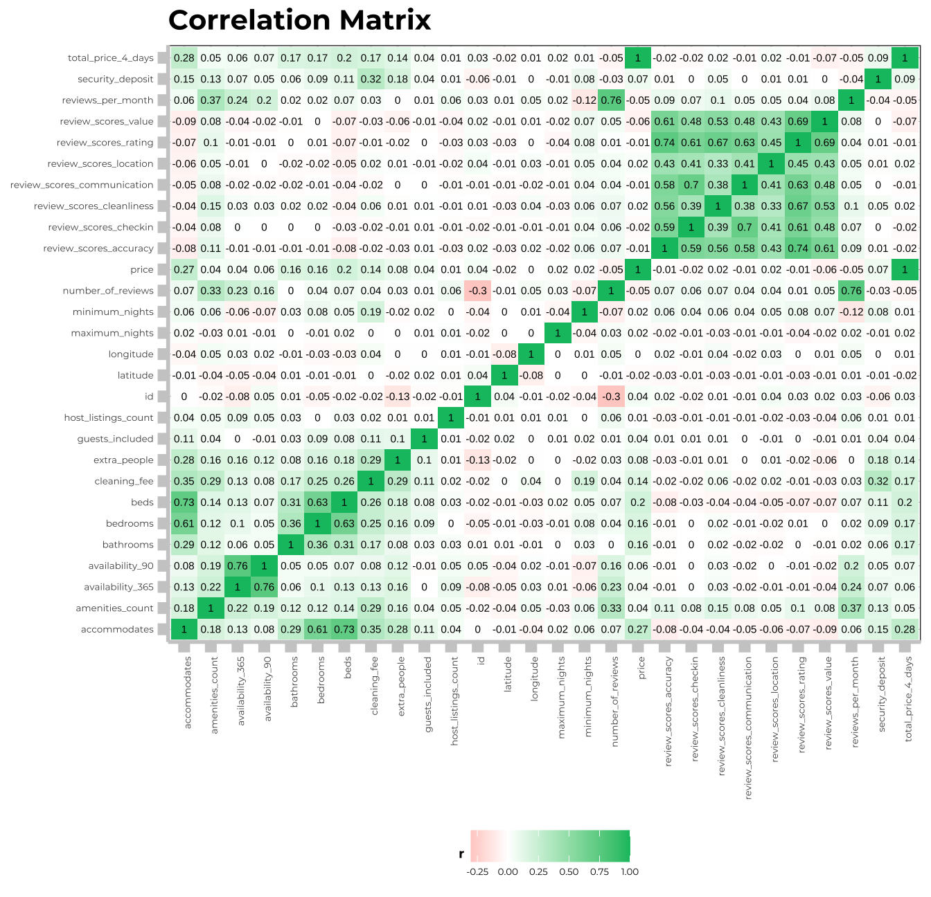
Further analysis for collinear variables
#munich_listing_is_numeric[,18:24]%>% #tried to spot the correlation between the review-related variables using ggpairs plot
#  ggpairs()

munich_listing_is_numeric%>% #used the ggpairs plot to further analyse the bottom left part of the correlation matrix
  select(accommodates,bathrooms,
         bedrooms,
         beds,
         cleaning_fee,
         extra_people,
         guests_included,
         total_price_4_days,
         security_deposit)%>%
  ggpairs()+
theme(panel.grid.major.y = element_line(color = "gray60", size = 0.2),
        strip.text= element_text(size=5, family="Montserrat", face = "bold"),
        panel.background = element_rect(fill = "white", colour = "white"),
        axis.line = element_line(size = 2, colour = "grey80"),
        axis.ticks = element_line(size = 3,colour = "grey80"),
        axis.ticks.length = unit(.20, "cm"),
        plot.title = element_text(color = "grey40",size=15,face="bold", family= "Montserrat"),
        plot.caption = element_text(color = "grey40", face="italic",size= 7,family= "Montserrat",hjust=0),
        axis.title.y = element_text(size = 4, angle = 90, family="Montserrat", face = "bold"),
        axis.text.y=element_text(family="Montserrat", size=4),
        axis.title.x = element_text(size = 4, family="Montserrat", face = "bold"),
        axis.text.x=element_text(family="Montserrat", size=4),
        legend.text=element_text(family="Montserrat", size=4),
        legend.title=element_text(family="Montserrat", size=4, face="bold"))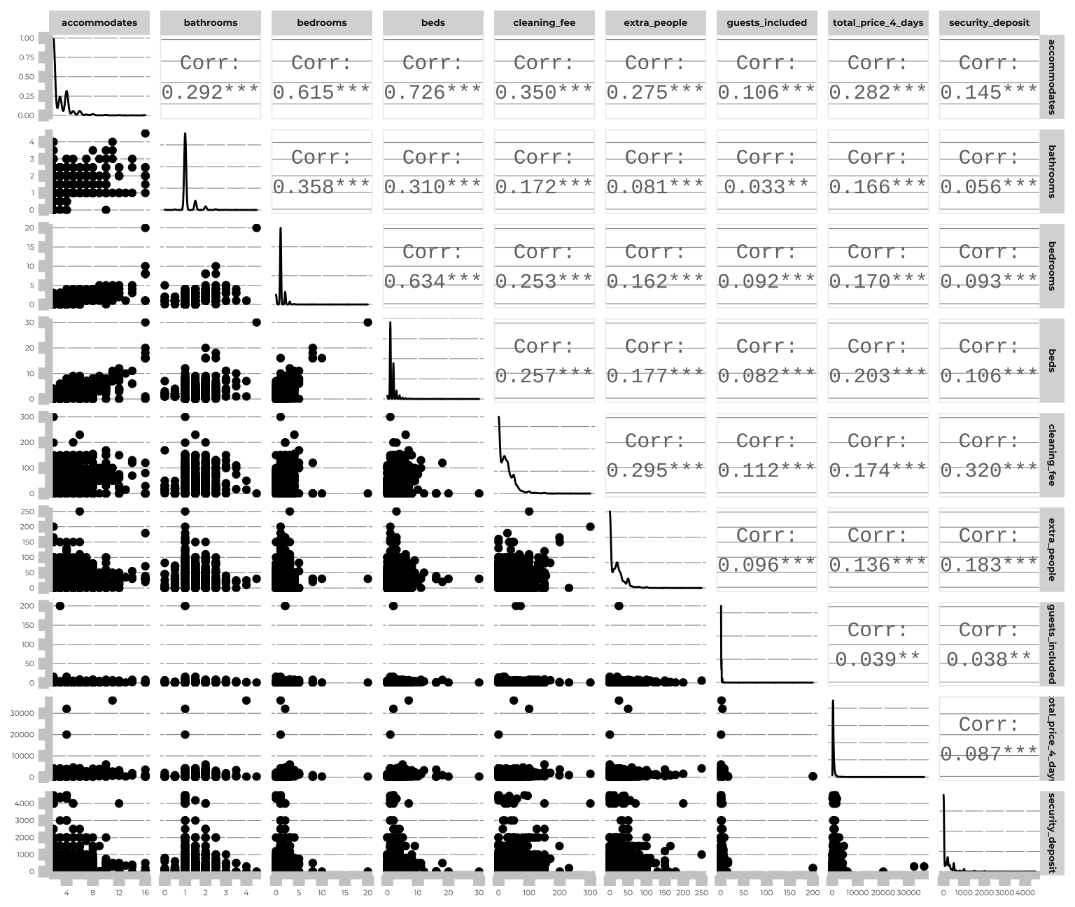
Key findings
The correlation matrix above displays two key ‘green zones’ where there are moderate to strong correlations present between variables. In the upper right corner, the plot illustrates the positive correlations between the various review score components, indicating that when an Airbnb scores well on one criterium it will tend to also have a higher rating on the other criteria. The strongest correlatio here is between the total review score and the review score for accuracy, at a level of 0.74. In the lower left corner we can see positive correlations between variables ranging from weak to strong. As one would expect, the number of people an Airbnb in Munich accomodates has a strong positive correlation with the number of beds and the number of bedrooms. There is a moderatore positive correlation between the total accomodated and the cleaning fee. Lastly, there is a moderate positive correlation between the cleaning fee and the security deposit, likely attributable to the fact that these properties are of a higher standard, as is mentioned on Airbnb’s website (deposits are usually based on a home’s features).
Looking at the independent variable of interest for this project, the total price for a 4-day stay for two people, I only find weak positive correlations when disregarding the obvious connection to daily price. With a level of 0.29 there is a weak to moderate positive correlation between the total price and the number of people an Airbnb can accommodate; this is further supported by weak correlations (0.22) between total price and the number of bedrooms and beds. I will now continue to investigate relationships between my variables, in particular categorical variables not included in the above matrix.
Informative visualisations
ggplot(listings,aes(x=number_of_reviews))+
  geom_histogram(binwidth = 4)+
    xlim(0,250)+
    ylim(0,1000)+
     labs(title="Most of the airbnb accomodations have up to 20 reviews",
          subtitle="Histrogram examining distribution of reviews",
          x="Number of Reviews",
          y="Quantity")+
  theme_bw()+
  theme(panel.background = element_rect(fill = "white", colour = "white"),
        axis.line = element_line(size = 1, colour = "grey80"),
        axis.ticks = element_line(size = 3,colour = "grey80"),
        axis.ticks.length = unit(.20, "cm"),
        plot.title = element_text(color = "black",size=12,face="bold", family= "Montserrat"),
        plot.subtitle = element_text(color = "black",size=10,face="plain", family= "Montserrat"),
        axis.title.y = element_text(size = 8, angle = 90, family="Montserrat", face = "plain"),
        axis.text.y=element_text(family="Montserrat", size=7),
        axis.title.x = element_text(size = 8, family="Montserrat", face = "plain"),
        axis.text.x=element_text(family="Montserrat", size=7),
        legend.text=element_text(family="Montserrat", size=7),
        legend.title=element_text(family="Montserrat", size=8, face="bold"))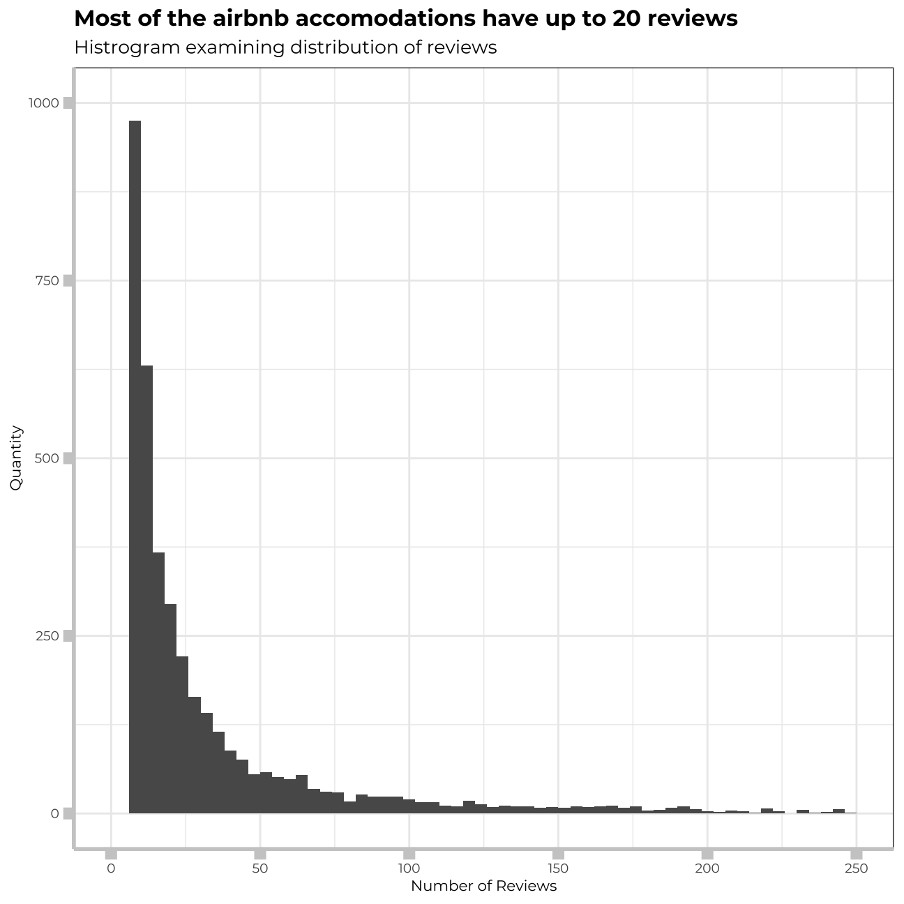
ggplot(munich_listing_is_numeric,
       aes(x=extra_people,y=total_price_4_days))+
  geom_point()+
  geom_smooth(method="lm")+
    ylim(0,3000)+
    xlim(0,100)+
      labs(title="Higher the Extra People Charge, the Higher the Overall Price",
           subtitle="Correlation between price per extra person and total price per 4 nights stay",
           x="Price per extra person",
           y="Total price for 4 nights")+
  theme_bw()+
    theme(panel.grid.major.y = element_line(color = "gray60", size = 0.1),
        panel.background = element_rect(fill = "white", colour = "white"),
        axis.line = element_line(size = 1, colour = "grey80"),
        axis.ticks = element_line(size = 3,colour = "grey80"),
        axis.ticks.length = unit(.20, "cm"),
        plot.title = element_text(color = "black",size=12,face="bold", family= "Montserrat"),
        plot.subtitle = element_text(color = "black",size=10,face="plain", family= "Montserrat"),
        axis.title.y = element_text(size = 8, angle = 90, family="Montserrat", face = "plain"),
        axis.text.y=element_text(family="Montserrat", size=7),
        axis.title.x = element_text(size = 8, family="Montserrat", face = "plain"),
        axis.text.x=element_text(family="Montserrat", size=7),
        legend.text=element_text(family="Montserrat", size=7),
        legend.title=element_text(family="Montserrat", size=8, face="bold"))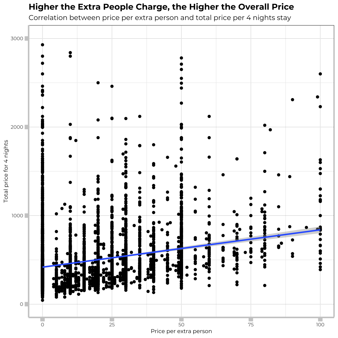
ggplot(munich_listings_region, aes(x=total_price_4_days))+
  geom_density(bins=20)+
  xlim(0,4000) +
  labs(title="The density plot of total price for 4 nights is heavily right-skwed",
       subtitle="Distribution of total price for 4 nights",
       x="Density",
       y="Total price for 4 nights")+
  theme_bw()+
    theme(panel.grid.major.y = element_line(color = "gray60", size = 0.1),
        panel.background = element_rect(fill = "white", colour = "white"),
        axis.line = element_line(size = 1, colour = "grey80"),
        axis.ticks = element_line(size = 3,colour = "grey80"),
        axis.ticks.length = unit(.20, "cm"),
        plot.title = element_text(color = "black",size=10,face="bold", family= "Montserrat"),
        plot.subtitle = element_text(color = "black",size=10,face="plain", family= "Montserrat"),
        axis.title.y = element_text(size = 8, angle = 90, family="Montserrat", face = "plain"),
        axis.text.y=element_text(family="Montserrat", size=7),
        axis.title.x = element_text(size = 8, family="Montserrat", face = "plain"),
        axis.text.x=element_text(family="Montserrat", size=7),
        legend.text=element_text(family="Montserrat", size=7),
        legend.title=element_text(family="Montserrat", size=8, face="bold"))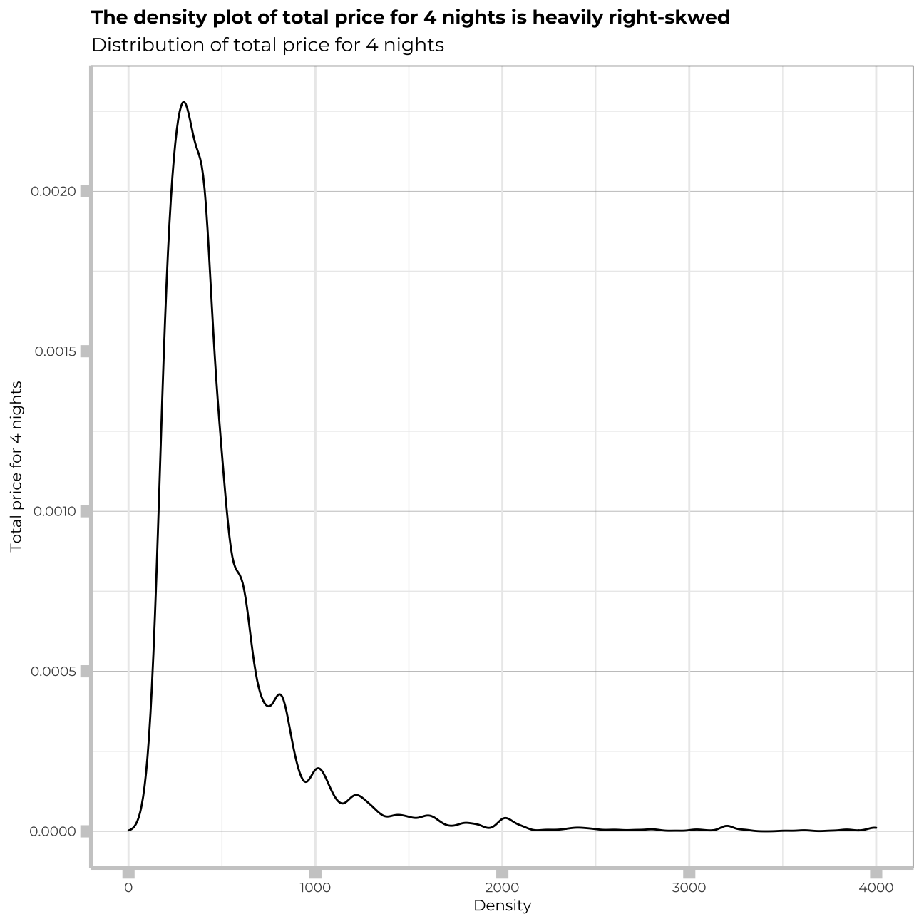
The distribution of price for 4 nights stay is heavilty right-skewed. I will examine now distribution of a logarithm of that price.
ggplot(munich_listings_total_price, aes(x=total_price_4_days))+
  geom_density(bins=20)+
  scale_x_log10()+
  xlim(0,2500) +
  labs(title="Logarithmic Total Price Shows Nature of Price Clusters",
              subtitle="Distribution of the log price for 4 nights stay",
       x="Density",
       y="Total price for 4 nights")+
  theme_bw()+
    theme(panel.grid.major.y = element_line(color = "gray60", size = 0.1),
        panel.background = element_rect(fill = "white", colour = "white"),
        axis.line = element_line(size = 1, colour = "grey80"),
        axis.ticks = element_line(size = 3,colour = "grey80"),
        axis.ticks.length = unit(.20, "cm"),
        plot.title = element_text(color = "black",size=12,face="bold", family= "Montserrat"),
        axis.title.y = element_text(size = 8, angle = 90, family="Montserrat", face = "plain"),
        axis.text.y=element_text(family="Montserrat", size=7),
        axis.title.x = element_text(size = 8, family="Montserrat", face = "plain"),
        axis.text.x=element_text(family="Montserrat", size=7),
        legend.text=element_text(family="Montserrat", size=7),
        legend.title=element_text(family="Montserrat", size=8, face="bold"))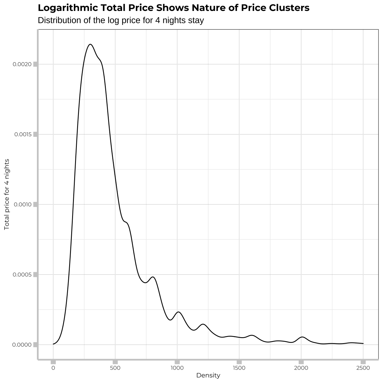
The log_price is heavily right-skewed as well.
ggplot(munich_listings_total_price, aes(x=total_price_4_days))+
  geom_histogram(bins=100)+
  xlim(0,2500)+
  labs(title="Most Airbnbs cost around €300 for 4 Nights",
       subtitle="Histogram of total price per 4 nights in Munich",
       x="Total price for 4 nights",
       y= "Quantity")+
  theme_bw()+
    theme(panel.grid.major.y = element_line(color = "gray60", size = 0.1),
        panel.background = element_rect(fill = "white", colour = "white"),
        axis.line = element_line(size = 1, colour = "grey80"),
        axis.ticks = element_line(size = 3,colour = "grey80"),
        axis.ticks.length = unit(.20, "cm"),
        plot.title = element_text(color = "black",size=12,face="bold", family= "Montserrat"),
        plot.subtitle = element_text(color = "black",size=10,face="plain", family= "Montserrat"),
        axis.title.y = element_text(size = 8, angle = 90, family="Montserrat", face = "plain"),
        axis.text.y=element_text(family="Montserrat", size=7),
        axis.title.x = element_text(size = 8, family="Montserrat", face = "plain"),
        axis.text.x=element_text(family="Montserrat", size=7),
        legend.text=element_text(family="Montserrat", size=7),
        legend.title=element_text(family="Montserrat", size=8, face="bold"))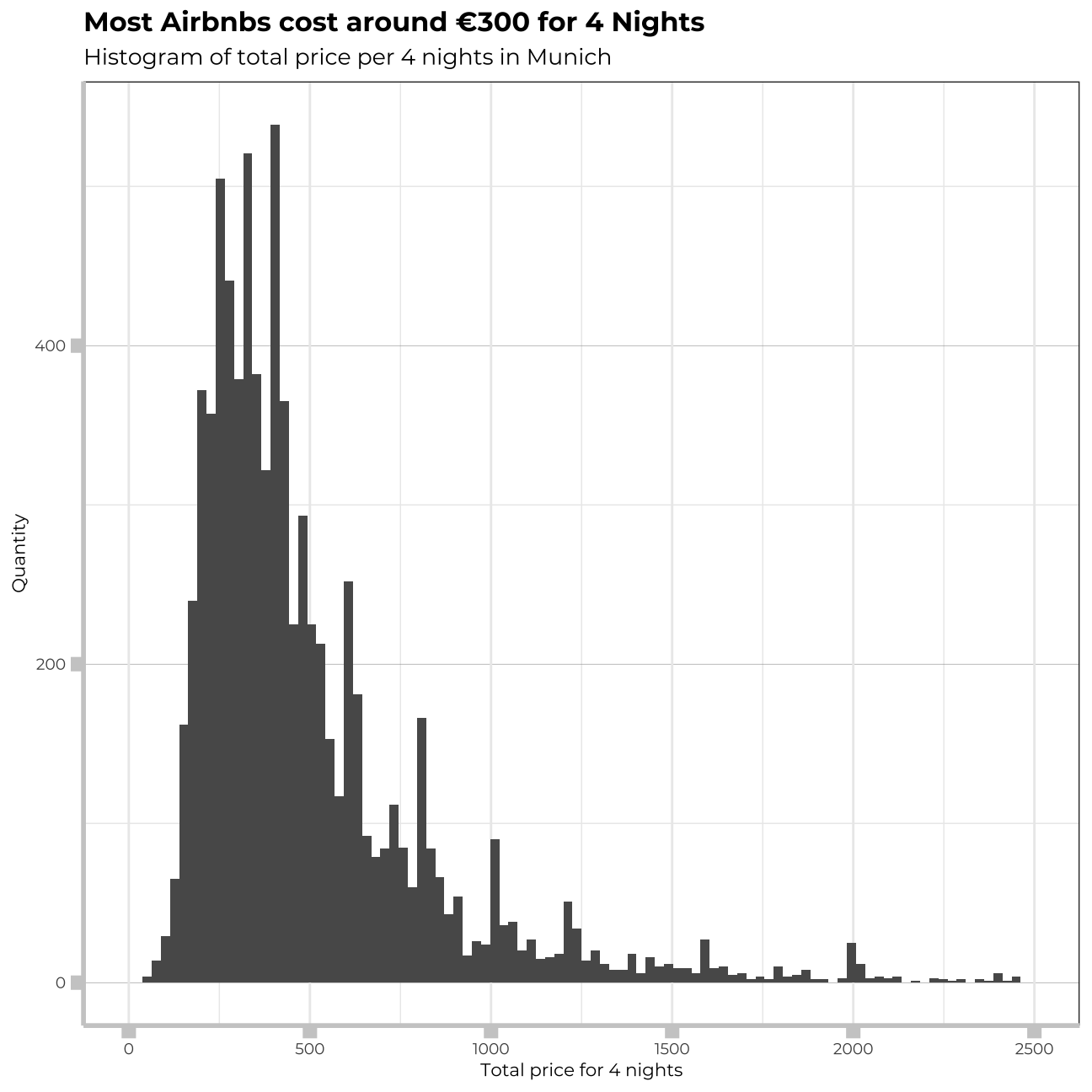
#Calculated mean price for 4 nights per room type
munich_listings_region %>%
  group_by(room_type) %>%
  summarize(mean_price_roomtype = mean(total_price_4_days)) %>%
  arrange(desc(mean_price_roomtype)) %>%
  ggplot(aes(y=reorder(room_type, mean_price_roomtype), x = mean_price_roomtype)) +
    geom_col() +
      labs(title="Hotel rooms are The Most Expensive Airbns in Munich",
           subtitle="Mean price for 4 night by room type",
           x="Average price for 4 nights per room",
           y="Room type")+
  theme_bw()+
    theme(panel.grid.major.y = element_line(color = "gray60", size = 0.1),
        panel.background = element_rect(fill = "white", colour = "white"),
        axis.line = element_line(size = 1, colour = "grey80"),
        axis.ticks = element_line(size = 3,colour = "grey80"),
        axis.ticks.length = unit(.20, "cm"),
        plot.title = element_text(color = "black",size=12,face="bold", family= "Montserrat"),
        plot.subtitle = element_text(color = "black",size=10,face="plain", family= "Montserrat"),
        axis.title.y = element_text(size = 8, angle = 90, family="Montserrat", face = "plain"),
        axis.text.y=element_text(family="Montserrat", size=7),
        axis.title.x = element_text(size = 8, family="Montserrat", face = "plain"),
        axis.text.x=element_text(family="Montserrat", size=7),
        legend.text=element_text(family="Montserrat", size=7),
        legend.title=element_text(family="Montserrat", size=8, face="bold"))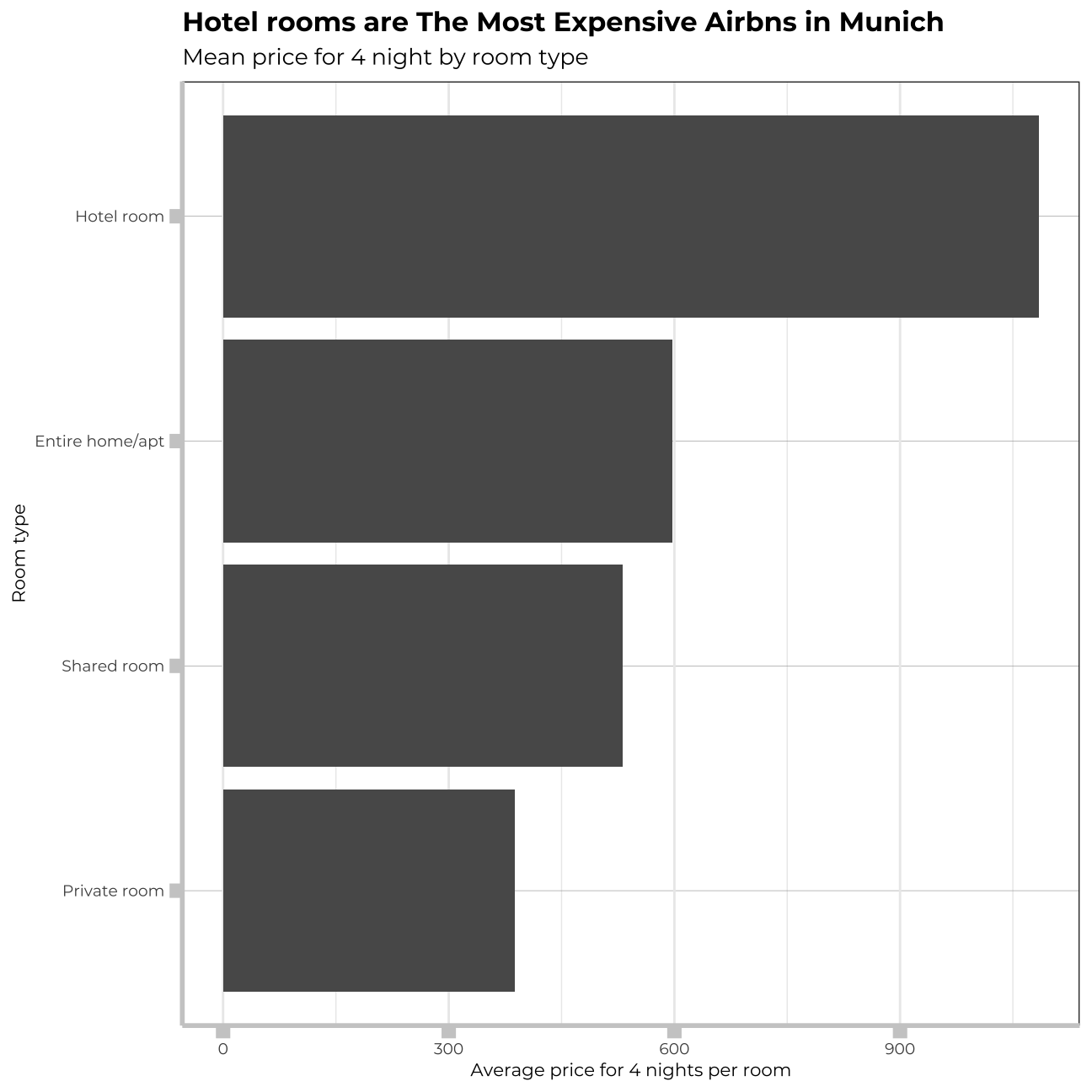
#Calculated mean price for 4 nights per neighbourhood
munich_listings_region %>%
  group_by(neighbourhood_cleansed) %>%
  summarize(mean_price_neighbourhood = mean(total_price_4_days)) %>%
  arrange(desc(mean_price_neighbourhood)) %>%
  ggplot(aes(y=reorder(neighbourhood_cleansed, mean_price_neighbourhood), x=mean_price_neighbourhood)) +
    geom_col()+
     labs(title="Average price for 4 nights per in particular neighbourhoods",
          x="Average price for per room",
          y="Neighbourhood")+
  theme_bw()+
  coord_flip()+
    theme(panel.grid.major.y = element_line(color = "gray60", size = 0.1),
        panel.background = element_rect(fill = "white", colour = "white"),
        axis.line = element_line(size = 1, colour = "grey80"),
        axis.ticks = element_line(size = 3,colour = "grey80"),
        axis.ticks.length = unit(.20, "cm"),
        plot.title = element_text(color = "black",size=12,face="bold", family= "Montserrat"),
        plot.subtitle = element_text(color = "black",size=10,face="plain", family= "Montserrat"),
        axis.title.y = element_text(size = 8, angle = 90, family="Montserrat", face = "plain"),
        axis.text.y=element_text(family="Montserrat", size=7),
        axis.title.x = element_text(size = 8, family="Montserrat",face = "plain"),
        axis.text.x=element_text(family="Montserrat", size=7,angle = 70, hjust = 1),
        legend.text=element_text(family="Montserrat", size=7),
        legend.title=element_text(family="Montserrat", size=8, face="bold"))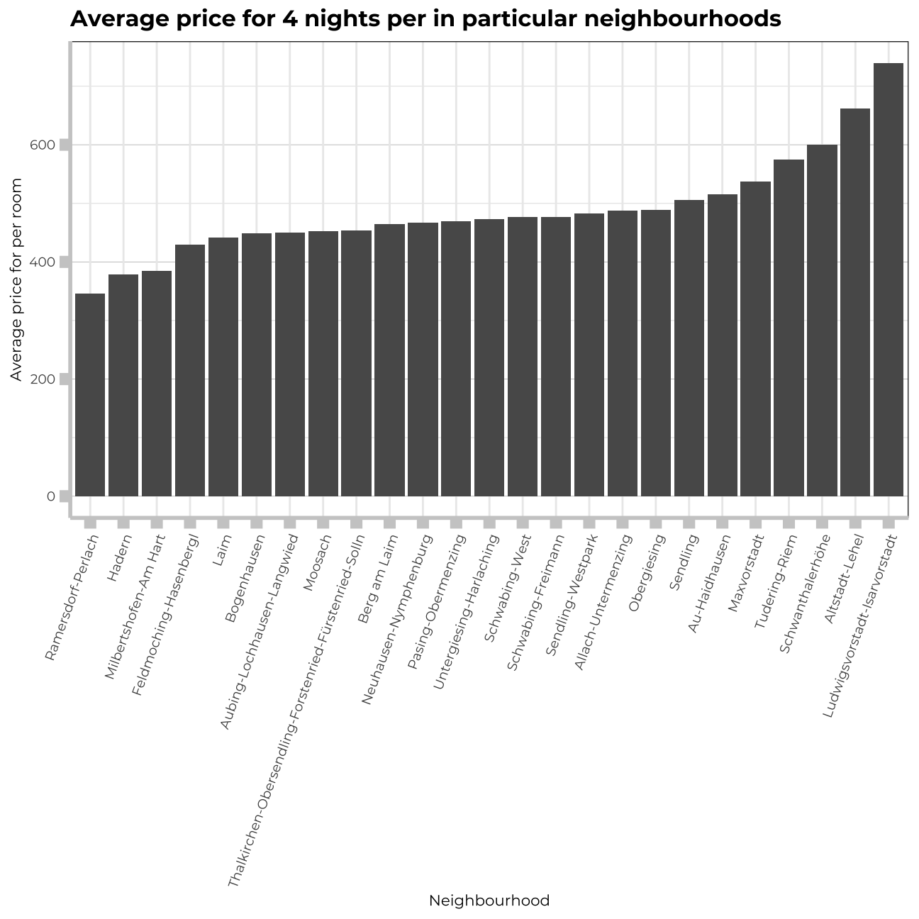
#Calculated mean price for 4 nights per property type
munich_listings_region %>%
  group_by(prop_type_simplified) %>%
  summarize(mean_price_property = mean(total_price_4_days)) %>%
  arrange(desc(mean_price_property)) %>%
  ggplot(aes(y=reorder(prop_type_simplified, mean_price_property), x = mean_price_property)) +
    geom_col() +
      labs(title="Lofts Come at a Premium in Munich, Houses Present\n a Good Value Proposition",
           x="Average price for per room",
           y="Property type")+
  theme_bw()+
    theme(panel.grid.major.y = element_line(color = "gray60", size = 0.1),
        panel.background = element_rect(fill = "white", colour = "white"),
        axis.line = element_line(size = 1, colour = "grey80"),
        axis.ticks = element_line(size = 3,colour = "grey80"),
        axis.ticks.length = unit(.20, "cm"),
        plot.title = element_text(color = "black",size=12,face="bold", family= "Montserrat"),
        axis.title.y = element_text(size = 8, angle = 90, family="Montserrat", face = "plain"),
        axis.text.y=element_text(family="Montserrat", size=7),
        axis.title.x = element_text(size = 8, family="Montserrat", face = "plain"),
        axis.text.x=element_text(family="Montserrat", size=7),
        legend.text=element_text(family="Montserrat", size=7),
        legend.title=element_text(family="Montserrat", size=8, face="bold"))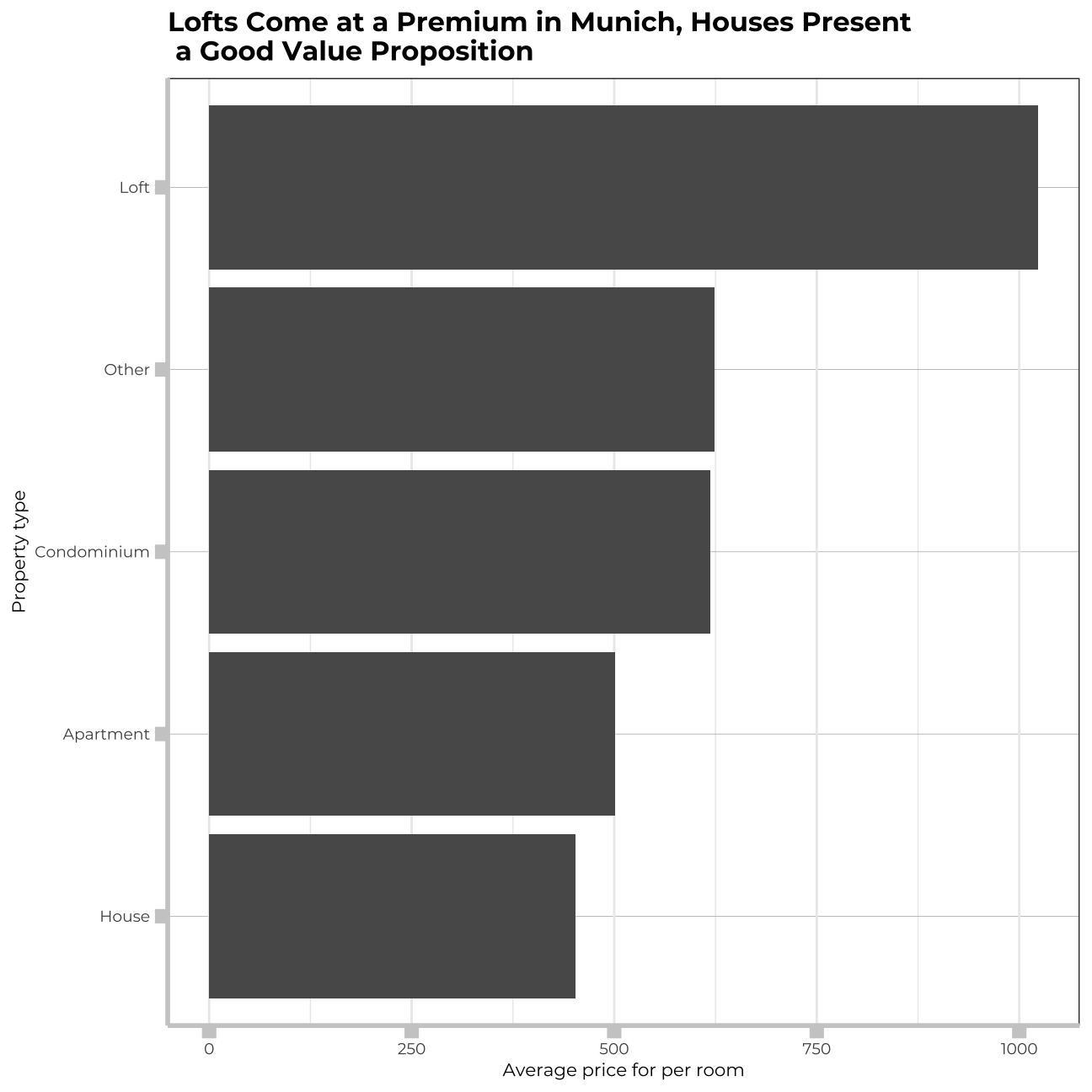
#Calculated count of particular property types
munich_listings_region %>%
  group_by(prop_type_simplified) %>%
  mutate(count_property=count("Apartment")) %>%
  arrange((count_property)) %>%
  ggplot(aes(x=reorder(prop_type_simplified, desc(count_property)), y = count_property)) +
    geom_col() +
      labs(title="Apartments Dominate Airbnb's Listings",
           x="Property type",
           y="Quantity")+
  theme_bw()+
    theme(panel.grid.major.y = element_line(color = "gray60", size = 0.1),
        panel.background = element_rect(fill = "white", colour = "white"),
        axis.line = element_line(size = 1, colour = "grey80"),
        axis.ticks = element_line(size = 3,colour = "grey80"),
        axis.ticks.length = unit(.20, "cm"),
        plot.title = element_text(color = "black",size=12,face="bold", family= "Montserrat"),
        axis.title.y = element_text(size = 8, angle = 90, family="Montserrat", face = "plain"),
        axis.text.y=element_text(family="Montserrat", size=7),
        axis.title.x = element_text(size = 8, family="Montserrat", face = "plain"),
        axis.text.x=element_text(family="Montserrat", size=7),
        legend.text=element_text(family="Montserrat", size=7),
        legend.title=element_text(family="Montserrat", size=8, face="bold"))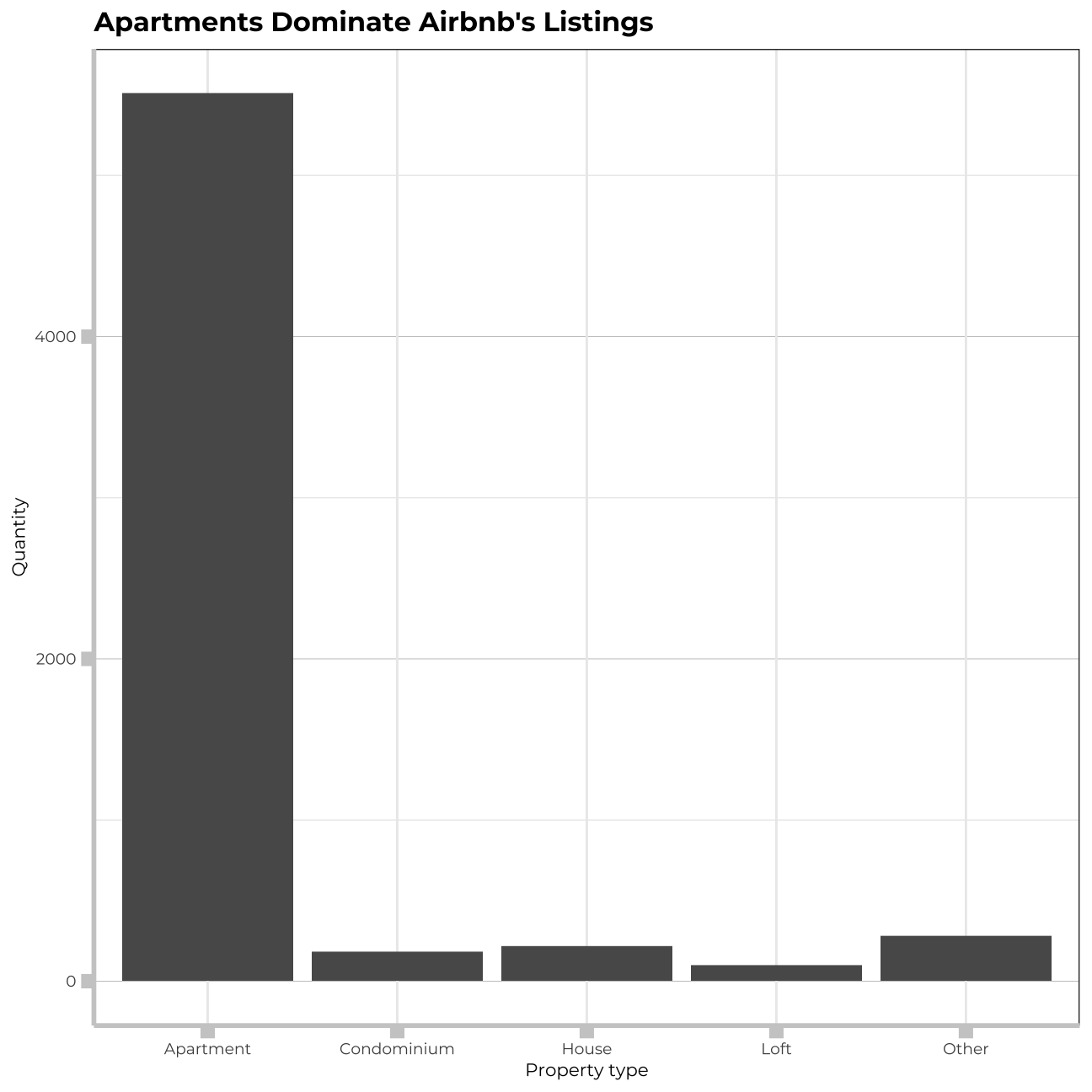
#Calculated average price for particular cancellation policies
munich_listings_region %>%
 group_by(cancellation_policy) %>%
  ggplot(aes(x=reorder(cancellation_policy,total_price_4_days ), y = total_price_4_days)) +
    geom_boxplot() +
      labs(title="Average prices per 4 nights for an Airbnb according to particular \ncancellation policies",
           y="Price",
           x="Cancellation policy")+
  scale_y_log10(limits=c(100,10000))+
  theme_bw()+
    theme(panel.grid.major.y = element_line(color = "gray60", size = 0.1),
        panel.background = element_rect(fill = "white", colour = "white"),
        axis.line = element_line(size = 1, colour = "grey80"),
        axis.ticks = element_line(size = 3,colour = "grey80"),
        axis.ticks.length = unit(.20, "cm"),
        plot.title = element_text(color = "black",size=12,face="bold", family= "Montserrat"),
        axis.title.y = element_text(size = 8, angle = 90, family="Montserrat", face = "plain"),
        axis.text.y=element_text(family="Montserrat", size=7),
        axis.title.x = element_text(size = 8, family="Montserrat", angle = 90,face = "plain"),
        axis.text.x=element_text(family="Montserrat", size=7),
        legend.text=element_text(family="Montserrat", size=7),
        legend.title=element_text(family="Montserrat", size=8, face="bold"))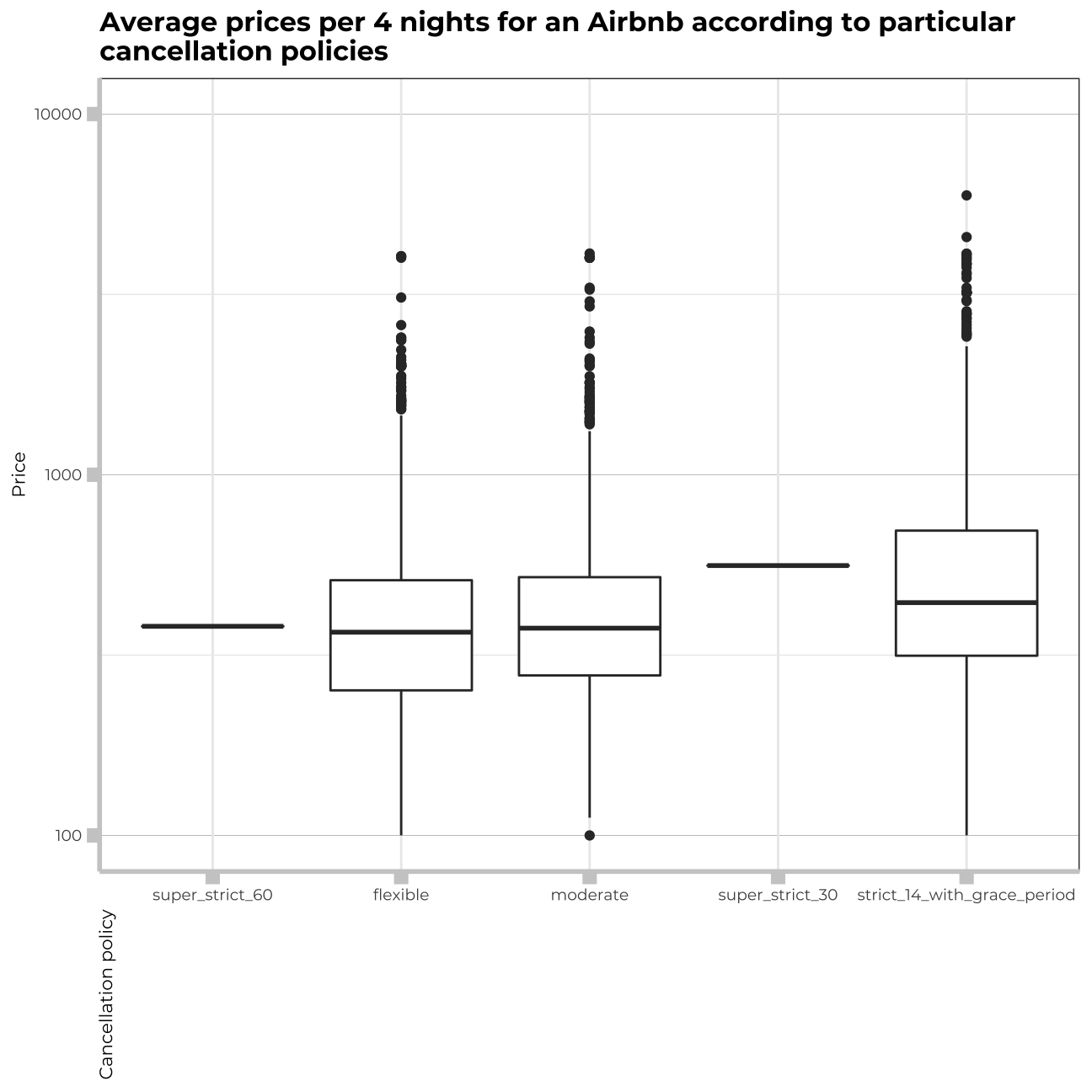
Mapping
Now, I will conduct the mapping of the Airbnbs’ locations on the Munich map. I decided to colour the data in regards to a particular zone they are located in, to have a better sense of the density of the accommodation in these zones. The zones were grouped by highest mean rental price, since it created the largest significance in our models later on.
pallette <- colorFactor(c("red", "blue", "green", "yellow","purple"), domain = c("zone_1", "zone_2", "zone_3", "zone_4","zone_5"))

    leaflet(data = munich_listings_region) %>%
  addProviderTiles("OpenStreetMap.Mapnik") %>%
  addCircleMarkers(lng = ~longitude,
                   lat = ~latitude,
                 radius = 2,
                 color = ~pallette(region),
                   fillColor = ~region,
                   group = ~ region,
                   clusterId=~region,
                   fillOpacity = 0.4,
                   popup = ~listing_url,
                   label = ~paste( prop_type_simplified, "Min nights", "=", minimum_nights))
Regression
Now I will start building my models. I will start from models with only a few variables and I will gradually try to build the model with the best fitting data and the biggest possible adjusted R-squared value. Running each model, I will as well check the colinearity analysis to cut confounding variables. For that reason I will use `car::vif(model_x)`` to calculate the Variance Inflation Factor (VIF) for our predictors. A general guideline is that a VIF larger than 5 or 10 is large, and the model may suffer from colinearity. I will remove the variable in question and run our model again without it if such a VIF occurs.
For my models I will use the log value of total_prices_4_days since the distribution of it is more bell shaped than the regular value and thus will be better descried by the model.
Model 1
I will fit our first regression model called model1 with the following explanatory variables: prop_type_simplified, number_of_reviews, and review_scores_rating.
#Regression using log because normally distributed.
model1 <-lm(log(total_price_4_days)~prop_type_simplified+
              number_of_reviews+
              review_scores_rating,
            data=munich_listings_region)
msummary(model1)
## Estimate Std. Error t value Pr(>|t|)
## (Intercept) 6.088376 0.082553 73.75 < 2e-16 ***
## prop_type_simplifiedCondominium 0.133395 0.044026 3.03 0.0025 **
## prop_type_simplifiedHouse -0.120477 0.040560 -2.97 0.0030 **
## prop_type_simplifiedLoft 0.303971 0.059575 5.10 3.5e-07 ***
## prop_type_simplifiedOther 0.105398 0.035956 2.93 0.0034 **
## number_of_reviews -0.001296 0.000154 -8.42 < 2e-16 ***
## review_scores_rating -0.000460 0.000867 -0.53 0.5958
##
## Residual standard error: 0.584 on 6278 degrees of freedom
## Multiple R-squared: 0.0185, Adjusted R-squared: 0.0176
## F-statistic: 19.7 on 6 and 6278 DF, p-value: <2e-16car::vif(model1)## GVIF Df GVIF^(1/(2*Df))
## prop_type_simplified 1.01 4 1
## number_of_reviews 1.01 1 1
## review_scores_rating 1.01 1 1#Noticed that variable review_scores_rating and "Other" and "House" categories
#in prop_type_simplified are also insignificant.
#Dropping review_scores_rating.After running model1, we can notice, that “review_scores_rating” is insignificant for the linear regression model as the p-value is bigger than 0.05.Therefore I will drop it. THe dummy variable “prop_type_simplified” turned out to be insignificant for Houses and Other property types. Anyway, I will keep the variable prop_type_simplified as some of it’s variables are important for our model. The Adjusted R-squared in this model is only 2,25%. I will try to fit more variables in our model in order to increase the accuracy.
I will add as well an example of interpretation of our data in logarithmic lm model.
The coefficient interpretation of review_scores_rating in regards to total_price_4_days is as follows: If the review_scores_rating increases by one, the total_price_4_days decreases by 0,0003%.
The coefficient interpretation of prop_type_simplified in regards to total_price_4_days is as follows: In regards to a particular property type the total_price_4_days behaves as follows: - (property type: Apartment) : total_price_4_days just takes the “Intercept” variable and increases by 6,08%. - (property type: Condominium) : prop_type_simplifiedCondominium=1; total_price_4_days increases by 0.18%. - (property type: House): prop_type_simplifiedHouse=1; total_price_4_days decreases by 0,065%. - (property type: Loft): prop_type_simplifiedLoft=1; total_price_4_days increases by 0.301%. - (property type: Other): prop_type_simplifiedOther=1; total_price_4_days increases by 0.06%.
Model 2
I want to determine if room_type is a significant predictor of the cost for 4 nights, given everything else in the model. I will fit a regression model that includes all of the explanatory variables in model1 plus room_type.
model2 <-lm(log(total_price_4_days)~prop_type_simplified+
              number_of_reviews+
              review_scores_rating+
              room_type,
            data=munich_listings_region)
msummary(model2)
## Estimate Std. Error t value Pr(>|t|)
## (Intercept) 6.149972 0.078743 78.10 < 2e-16 ***
## prop_type_simplifiedCondominium 0.102904 0.041903 2.46 0.01409 *
## prop_type_simplifiedHouse 0.034654 0.039001 0.89 0.37429
## prop_type_simplifiedLoft 0.215260 0.056691 3.80 0.00015 ***
## prop_type_simplifiedOther 0.118736 0.036437 3.26 0.00113 **
## number_of_reviews -0.001216 0.000146 -8.32 < 2e-16 ***
## review_scores_rating 0.000413 0.000827 0.50 0.61778
## room_typeHotel room 0.296750 0.101852 2.91 0.00359 **
## room_typePrivate room -0.376066 0.014681 -25.62 < 2e-16 ***
## room_typeShared room -0.252149 0.063355 -3.98 7e-05 ***
##
## Residual standard error: 0.554 on 6275 degrees of freedom
## Multiple R-squared: 0.115, Adjusted R-squared: 0.114
## F-statistic: 90.8 on 9 and 6275 DF, p-value: <2e-16car::vif(model2)## GVIF Df GVIF^(1/(2*Df))
## prop_type_simplified 1.19 4 1.02
## number_of_reviews 1.01 1 1.00
## review_scores_rating 1.01 1 1.01
## room_type 1.19 3 1.03The room_type has increased our adjusted R-squared up to 0.13. The p-value for each room type is less than 0,05, thus the room type variable is important and we will keep it in our model.
Model 3
Are the number of bathrooms, bedrooms, beds, or size of the house (accommodates) significant predictors of price_4_nights?
model3 <-lm(log(total_price_4_days)~prop_type_simplified+
              number_of_reviews+
              room_type+
              bathrooms+
              bedrooms+
              beds+
              accommodates,
            data=munich_listings_region)
msummary(model3)
## Estimate Std. Error t value Pr(>|t|)
## (Intercept) 5.572998 0.026251 212.30 < 2e-16 ***
## prop_type_simplifiedCondominium 0.071778 0.038345 1.87 0.06126 .
## prop_type_simplifiedHouse -0.111393 0.036073 -3.09 0.00202 **
## prop_type_simplifiedLoft 0.115665 0.052001 2.22 0.02616 *
## prop_type_simplifiedOther 0.001071 0.033556 0.03 0.97455
## number_of_reviews -0.001522 0.000134 -11.36 < 2e-16 ***
## room_typeHotel room 0.539684 0.093272 5.79 7.5e-09 ***
## room_typePrivate room -0.248913 0.014236 -17.48 < 2e-16 ***
## room_typeShared room -0.296707 0.057856 -5.13 3.0e-07 ***
## bathrooms 0.124320 0.023376 5.32 1.1e-07 ***
## bedrooms 0.048444 0.012833 3.77 0.00016 ***
## beds -0.025160 0.008086 -3.11 0.00187 **
## accommodates 0.148472 0.006718 22.10 < 2e-16 ***
##
## Residual standard error: 0.506 on 6272 degrees of freedom
## Multiple R-squared: 0.263, Adjusted R-squared: 0.261
## F-statistic: 186 on 12 and 6272 DF, p-value: <2e-16car::vif(model3)## GVIF Df GVIF^(1/(2*Df))
## prop_type_simplified 1.26 4 1.03
## number_of_reviews 1.02 1 1.01
## room_type 1.35 3 1.05
## bathrooms 1.21 1 1.10
## bedrooms 1.93 1 1.39
## beds 2.45 1 1.57
## accommodates 2.50 1 1.58All the variables in our model apart from “beds” variable ware significant as t-value of these variables is more than 2. In our further models we will keep “bedrooms”, “bathrooms” and “accommodates”, however I will drop the “beds” as they are correlated to other variables.
Model 4
Do superhosts (host_is_superhost) command a pricing premium, after controlling for other variables?
model4 <-lm(log(total_price_4_days)~prop_type_simplified+
              number_of_reviews+
              room_type+
              bathrooms+
              bedrooms+
              accommodates+
              host_is_superhost,
            data=munich_listings_region)
msummary(model4)
## Estimate Std. Error t value Pr(>|t|)
## (Intercept) 5.58557 0.02604 214.49 < 2e-16 ***
## prop_type_simplifiedCondominium 0.06643 0.03833 1.73 0.0831 .
## prop_type_simplifiedHouse -0.11569 0.03607 -3.21 0.0013 **
## prop_type_simplifiedLoft 0.11464 0.05205 2.20 0.0277 *
## prop_type_simplifiedOther -0.00874 0.03343 -0.26 0.7938
## number_of_reviews -0.00150 0.00014 -10.71 < 2e-16 ***
## room_typeHotel room 0.54283 0.09335 5.81 6.4e-09 ***
## room_typePrivate room -0.24687 0.01427 -17.30 < 2e-16 ***
## room_typeShared room -0.30343 0.05787 -5.24 1.6e-07 ***
## bathrooms 0.11950 0.02334 5.12 3.1e-07 ***
## bedrooms 0.03550 0.01215 2.92 0.0035 **
## accommodates 0.13772 0.00576 23.92 < 2e-16 ***
## host_is_superhostTRUE -0.01540 0.01827 -0.84 0.3995
##
## Residual standard error: 0.507 on 6272 degrees of freedom
## Multiple R-squared: 0.262, Adjusted R-squared: 0.26
## F-statistic: 185 on 12 and 6272 DF, p-value: <2e-16car::vif(model4)## GVIF Df GVIF^(1/(2*Df))
## prop_type_simplified 1.25 4 1.03
## number_of_reviews 1.10 1 1.05
## room_type 1.35 3 1.05
## bathrooms 1.21 1 1.10
## bedrooms 1.73 1 1.32
## accommodates 1.83 1 1.35
## host_is_superhost 1.10 1 1.05Superhosts do not command a pricing premium in Munich, therefore I will drop this variable in our further models. I can see that the VIF for bedrooms and accommodates has a bit higher VIF, however it is still not high enough to worry about it.
Model 5
Most owners advertise the exact location of their listing (is_location_exact == TRUE), while a non-trivial proportion don’t.
After controlling for other variables, is a listing’s exact location a significant predictor of price_4_nights?
model5 <-lm(log(total_price_4_days)~prop_type_simplified+
              number_of_reviews+
              room_type+bathrooms+
              bedrooms+accommodates+
              is_location_exact,
            data=munich_listings_region)
msummary(model5)
## Estimate Std. Error t value Pr(>|t|)
## (Intercept) 5.581474 0.028604 195.13 < 2e-16 ***
## prop_type_simplifiedCondominium 0.066161 0.038340 1.73 0.0845 .
## prop_type_simplifiedHouse -0.116372 0.036065 -3.23 0.0013 **
## prop_type_simplifiedLoft 0.113322 0.052045 2.18 0.0295 *
## prop_type_simplifiedOther -0.008855 0.033432 -0.26 0.7911
## number_of_reviews -0.001531 0.000134 -11.41 < 2e-16 ***
## room_typeHotel room 0.541088 0.093351 5.80 7.1e-09 ***
## room_typePrivate room -0.247594 0.014245 -17.38 < 2e-16 ***
## room_typeShared room -0.302153 0.057904 -5.22 1.9e-07 ***
## bathrooms 0.119077 0.023355 5.10 3.5e-07 ***
## bedrooms 0.035545 0.012156 2.92 0.0035 **
## accommodates 0.137657 0.005757 23.91 < 2e-16 ***
## is_location_exactTRUE 0.004097 0.016237 0.25 0.8008
##
## Residual standard error: 0.507 on 6272 degrees of freedom
## Multiple R-squared: 0.262, Adjusted R-squared: 0.26
## F-statistic: 185 on 12 and 6272 DF, p-value: <2e-16car::vif(model5)## GVIF Df GVIF^(1/(2*Df))
## prop_type_simplified 1.24 4 1.03
## number_of_reviews 1.02 1 1.01
## room_type 1.35 3 1.05
## bathrooms 1.21 1 1.10
## bedrooms 1.73 1 1.32
## accommodates 1.83 1 1.35
## is_location_exact 1.01 1 1.00The variable “is_location_exact” does not have a significant influence on the price of an Airbnb in Munich (p-value bigger than 0.05). Therefore, I will drop it.
Model 6
Now I will use a variable that I created - "region" that clusters all the neighbourhood to 5 zones and I will see how the location affects the price for Airbnb in the model.
model6 <-lm(log(total_price_4_days)~prop_type_simplified+
              number_of_reviews+
              room_type+
              bathrooms+
              bedrooms+
              accommodates+
              region,
            data=munich_listings_region)
msummary(model6)
## Estimate Std. Error t value Pr(>|t|)
## (Intercept) 5.714978 0.027012 211.57 < 2e-16 ***
## prop_type_simplifiedCondominium 0.060742 0.037425 1.62 0.1046
## prop_type_simplifiedHouse -0.054203 0.035507 -1.53 0.1269
## prop_type_simplifiedLoft 0.113490 0.050802 2.23 0.0255 *
## prop_type_simplifiedOther 0.001530 0.032756 0.05 0.9628
## number_of_reviews -0.001616 0.000131 -12.34 < 2e-16 ***
## room_typeHotel room 0.497268 0.091203 5.45 5.2e-08 ***
## room_typePrivate room -0.234415 0.013930 -16.83 < 2e-16 ***
## room_typeShared room -0.284806 0.056523 -5.04 4.8e-07 ***
## bathrooms 0.118175 0.022790 5.19 2.2e-07 ***
## bedrooms 0.038658 0.011872 3.26 0.0011 **
## accommodates 0.137573 0.005620 24.48 < 2e-16 ***
## regionzone_2 -0.139446 0.016825 -8.29 < 2e-16 ***
## regionzone_3 -0.195816 0.018061 -10.84 < 2e-16 ***
## regionzone_4 -0.198716 0.022296 -8.91 < 2e-16 ***
## regionzone_5 -0.334734 0.020304 -16.49 < 2e-16 ***
##
## Residual standard error: 0.495 on 6269 degrees of freedom
## Multiple R-squared: 0.297, Adjusted R-squared: 0.295
## F-statistic: 176 on 15 and 6269 DF, p-value: <2e-16car::vif(model6)## GVIF Df GVIF^(1/(2*Df))
## prop_type_simplified 1.28 4 1.03
## number_of_reviews 1.02 1 1.01
## room_type 1.36 3 1.05
## bathrooms 1.21 1 1.10
## bedrooms 1.73 1 1.32
## accommodates 1.83 1 1.35
## region 1.04 4 1.00The region of Munich has a significant influence on the price. T-value of all the zone is way more than |2| and our adjusted R-squared went up - it suggests that model 6 better describes the real data than our previous models.
Model 7
What is the effect of cancellation_policy on price_4_nights, after I control for other variables?
model7 <-lm(log(total_price_4_days)~prop_type_simplified+
              number_of_reviews+
              room_type+
              bathrooms+
              bedrooms+
              accommodates+
              region+
              cancellation_policy,
            data=munich_listings_region)
msummary(model7)
## Estimate Std. Error t value
## (Intercept) 5.68179 0.02810 202.18
## prop_type_simplifiedCondominium 0.04985 0.03715 1.34
## prop_type_simplifiedHouse -0.06235 0.03524 -1.77
## prop_type_simplifiedLoft 0.11069 0.05041 2.20
## prop_type_simplifiedOther 0.01612 0.03253 0.50
## number_of_reviews -0.00168 0.00013 -12.87
## room_typeHotel room 0.50907 0.09051 5.62
## room_typePrivate room -0.22810 0.01388 -16.43
## room_typeShared room -0.29699 0.05610 -5.29
## bathrooms 0.11434 0.02262 5.06
## bedrooms 0.04181 0.01179 3.55
## accommodates 0.13068 0.00562 23.26
## regionzone_2 -0.13437 0.01670 -8.05
## regionzone_3 -0.18655 0.01795 -10.39
## regionzone_4 -0.19215 0.02213 -8.68
## regionzone_5 -0.32519 0.02018 -16.12
## cancellation_policymoderate 0.00772 0.01509 0.51
## cancellation_policystrict_14_with_grace_period 0.14262 0.01565 9.11
## cancellation_policysuper_strict_30 0.13203 0.49206 0.27
## cancellation_policysuper_strict_60 0.02713 0.49100 0.06
## Pr(>|t|)
## (Intercept) < 2e-16 ***
## prop_type_simplifiedCondominium 0.17960
## prop_type_simplifiedHouse 0.07691 .
## prop_type_simplifiedLoft 0.02813 *
## prop_type_simplifiedOther 0.62028
## number_of_reviews < 2e-16 ***
## room_typeHotel room 1.9e-08 ***
## room_typePrivate room < 2e-16 ***
## room_typeShared room 1.2e-07 ***
## bathrooms 4.4e-07 ***
## bedrooms 0.00039 ***
## accommodates < 2e-16 ***
## regionzone_2 1.0e-15 ***
## regionzone_3 < 2e-16 ***
## regionzone_4 < 2e-16 ***
## regionzone_5 < 2e-16 ***
## cancellation_policymoderate 0.60895
## cancellation_policystrict_14_with_grace_period < 2e-16 ***
## cancellation_policysuper_strict_30 0.78846
## cancellation_policysuper_strict_60 0.95594
##
## Residual standard error: 0.491 on 6265 degrees of freedom
## Multiple R-squared: 0.308, Adjusted R-squared: 0.306
## F-statistic: 147 on 19 and 6265 DF, p-value: <2e-16car::vif(model7)## GVIF Df GVIF^(1/(2*Df))
## prop_type_simplified 1.28 4 1.03
## number_of_reviews 1.03 1 1.01
## room_type 1.37 3 1.05
## bathrooms 1.21 1 1.10
## bedrooms 1.74 1 1.32
## accommodates 1.86 1 1.36
## region 1.05 4 1.01
## cancellation_policy 1.06 4 1.01The cancellation policy of 14 days seems to have a significant impact on the price for 4 nights. This is why I will keep the variable “cancellation policy” in my model. The Adjusted R-squared again went up by one percent. Let me keep trying adding more variables that may turn out significant for the model.
Final Model
Now I will create the model with numerous significant data that I checked to be relevant and significant to create our best fitting regression model.
model_wild_west<-lm(log10(total_price_4_days)~ #predicting total_price_4_days on variables below
                      prop_type_simplified+
                      number_of_reviews* #multiplied because of colinearity
                      reviews_per_month+
                      room_type*  # multiplied because of colinearity
                      bedrooms+
                      bathrooms+
                      accommodates+
                      region+
                      cancellation_policy+
                      review_scores_value+
                      review_scores_cleanliness+
                      review_scores_checkin+
                      review_scores_location+
                      security_deposit+
                      rating_group+
                      instant_bookable+
                      availability_365+
                      availability_90+
                      maximum_nights+
                      minimum_nights+
                      is_elevator+
                      is_shampoo,
                    data=munich_listings_region)
msummary(model_wild_west)
## Estimate Std. Error t value
## (Intercept) 2.36e+00 5.15e-02 45.75
## prop_type_simplifiedCondominium 1.73e-02 1.52e-02 1.14
## prop_type_simplifiedHouse -2.75e-02 1.47e-02 -1.87
## prop_type_simplifiedLoft 4.35e-02 2.07e-02 2.10
## prop_type_simplifiedOther 1.35e-02 1.36e-02 1.00
## number_of_reviews -1.02e-03 1.26e-04 -8.09
## reviews_per_month -4.82e-02 3.91e-03 -12.33
## room_typeHotel room 2.78e-01 6.37e-02 4.36
## room_typePrivate room -1.36e-03 1.06e-02 -0.13
## room_typeShared room -1.44e-01 2.32e-02 -6.20
## bedrooms 5.34e-02 5.46e-03 9.78
## bathrooms 4.79e-02 9.29e-03 5.16
## accommodates 5.04e-02 2.33e-03 21.66
## regionzone_2 -5.87e-02 6.86e-03 -8.56
## regionzone_3 -7.87e-02 7.42e-03 -10.61
## regionzone_4 -8.15e-02 9.12e-03 -8.94
## regionzone_5 -1.30e-01 8.45e-03 -15.38
## cancellation_policymoderate 8.61e-03 6.25e-03 1.38
## cancellation_policystrict_14_with_grace_period 4.86e-02 6.56e-03 7.40
## cancellation_policysuper_strict_30 -4.57e-02 2.01e-01 -0.23
## cancellation_policysuper_strict_60 -6.72e-02 2.01e-01 -0.33
## review_scores_value -4.56e-02 3.41e-03 -13.38
## review_scores_cleanliness 2.14e-02 3.24e-03 6.61
## review_scores_checkin 1.17e-02 4.18e-03 2.79
## review_scores_location 2.15e-02 4.18e-03 5.14
## security_deposit 4.85e-05 7.24e-06 6.71
## rating_groupUnder 90 -3.34e-02 9.15e-03 -3.65
## instant_bookableTRUE 3.78e-02 5.66e-03 6.67
## availability_365 1.47e-04 3.51e-05 4.20
## availability_90 6.93e-04 1.09e-04 6.35
## maximum_nights 3.67e-06 1.57e-06 2.33
## minimum_nights -1.63e-02 3.20e-03 -5.09
## is_elevatorTRUE 1.09e-02 5.29e-03 2.07
## is_shampooTRUE 1.13e-02 5.27e-03 2.13
## number_of_reviews:reviews_per_month 1.90e-04 2.41e-05 7.89
## room_typeHotel room:bedrooms -1.04e-01 4.79e-02 -2.17
## room_typePrivate room:bedrooms -1.03e-01 8.24e-03 -12.47
## Pr(>|t|)
## (Intercept) < 2e-16 ***
## prop_type_simplifiedCondominium 0.25581
## prop_type_simplifiedHouse 0.06090 .
## prop_type_simplifiedLoft 0.03548 *
## prop_type_simplifiedOther 0.31864
## number_of_reviews 7.0e-16 ***
## reviews_per_month < 2e-16 ***
## room_typeHotel room 1.3e-05 ***
## room_typePrivate room 0.89790
## room_typeShared room 6.1e-10 ***
## bedrooms < 2e-16 ***
## bathrooms 2.6e-07 ***
## accommodates < 2e-16 ***
## regionzone_2 < 2e-16 ***
## regionzone_3 < 2e-16 ***
## regionzone_4 < 2e-16 ***
## regionzone_5 < 2e-16 ***
## cancellation_policymoderate 0.16853
## cancellation_policystrict_14_with_grace_period 1.5e-13 ***
## cancellation_policysuper_strict_30 0.82010
## cancellation_policysuper_strict_60 0.73774
## review_scores_value < 2e-16 ***
## review_scores_cleanliness 4.2e-11 ***
## review_scores_checkin 0.00526 **
## review_scores_location 2.8e-07 ***
## security_deposit 2.2e-11 ***
## rating_groupUnder 90 0.00026 ***
## instant_bookableTRUE 2.7e-11 ***
## availability_365 2.7e-05 ***
## availability_90 2.2e-10 ***
## maximum_nights 0.01965 *
## minimum_nights 3.7e-07 ***
## is_elevatorTRUE 0.03885 *
## is_shampooTRUE 0.03289 *
## number_of_reviews:reviews_per_month 3.5e-15 ***
## room_typeHotel room:bedrooms 0.02973 *
## room_typePrivate room:bedrooms < 2e-16 ***
##
## Residual standard error: 0.2 on 6248 degrees of freedom
## Multiple R-squared: 0.391, Adjusted R-squared: 0.387
## F-statistic: 111 on 36 and 6248 DF, p-value: <2e-16model_wild_west_colinear<-lm(log10(total_price_4_days)~ #predicting total_price_4_days on variables below
prop_type_simplified+
number_of_reviews+ #linearised for colinearity
reviews_per_month+
room_type+ # linearised for colinearity
bedrooms+
bathrooms+
accommodates+
region+
cancellation_policy+
review_scores_value+
review_scores_cleanliness+
review_scores_checkin+
review_scores_location+
security_deposit+
rating_group+
instant_bookable+
availability_365+
availability_90+
maximum_nights+
minimum_nights+
is_elevator+
is_shampoo,
data=munich_listings_region)
car::vif(model_wild_west_colinear) # car VIF struggles with multiplied variables so a new unmultiplied model is used to check.## GVIF Df GVIF^(1/(2*Df))
## prop_type_simplified 1.39 4 1.04
## number_of_reviews 2.45 1 1.56
## reviews_per_month 2.60 1 1.61
## room_type 1.60 3 1.08
## bedrooms 1.77 1 1.33
## bathrooms 1.22 1 1.11
## accommodates 1.91 1 1.38
## region 1.12 4 1.01
## cancellation_policy 1.14 4 1.02
## review_scores_value 1.79 1 1.34
## review_scores_cleanliness 1.69 1 1.30
## review_scores_checkin 1.48 1 1.22
## review_scores_location 1.41 1 1.19
## security_deposit 1.07 1 1.03
## rating_group 1.62 1 1.27
## instant_bookable 1.09 1 1.04
## availability_365 2.50 1 1.58
## availability_90 2.38 1 1.54
## maximum_nights 1.02 1 1.01
## minimum_nights 1.15 1 1.07
## is_elevator 1.07 1 1.03
## is_shampoo 1.05 1 1.03In the final model I tested variables from the previous models that were significant and tested much more variables that in my opinion could as well affect the total_price_4_days. I tested the variables connected to review scores - i.e. review_scores_value, review_scores_cleanliness, review_scores_checking_ review_scores_location etc. Only the ones mentioned turned out to be significant for the model.
Afterwards I checked for security_deposit, rating_group, instants_bookable and availability variables. Two of them (availability_60 and availability_30) turned out to be insignificant, so I decided to drop them.
Thereafter, I added host_listings_count as I believe that the number of properties the host has may affect the standard, build some economies of scales perhaps and therefore affect somehow the price. This factor as well turned out to be significant.
Later I tested maximum_nights and minimum_nights. In the next step I was testing whether particular types of amenities have any significant impact on the price. It turned out that two of them - elevator and shampoo (as they are always part of some welcome packs) are also significant for the price’s prediction. Moreover, I added two interaction variables - room_type&bedrooms and number_of_reviews&review_per_month as I believe there is much interaction happening between them. The final model has adjusted R-squared at the level of 38.7% and a RSE at the level of 0.2. Checking the VIF throughout, I can see that the GVIF value is well below 5 and we can be assured that the colinearity is not affecting the model significantly.
Diagnostics
Checking Residuals
In the next step I will plot residuals, analyze their behaviour and check whether they are distributed within the norms. Afterwards I will compare all the models and compare how they evolved.
#plotting residuals
autoplot(model_wild_west)+
  theme_bw()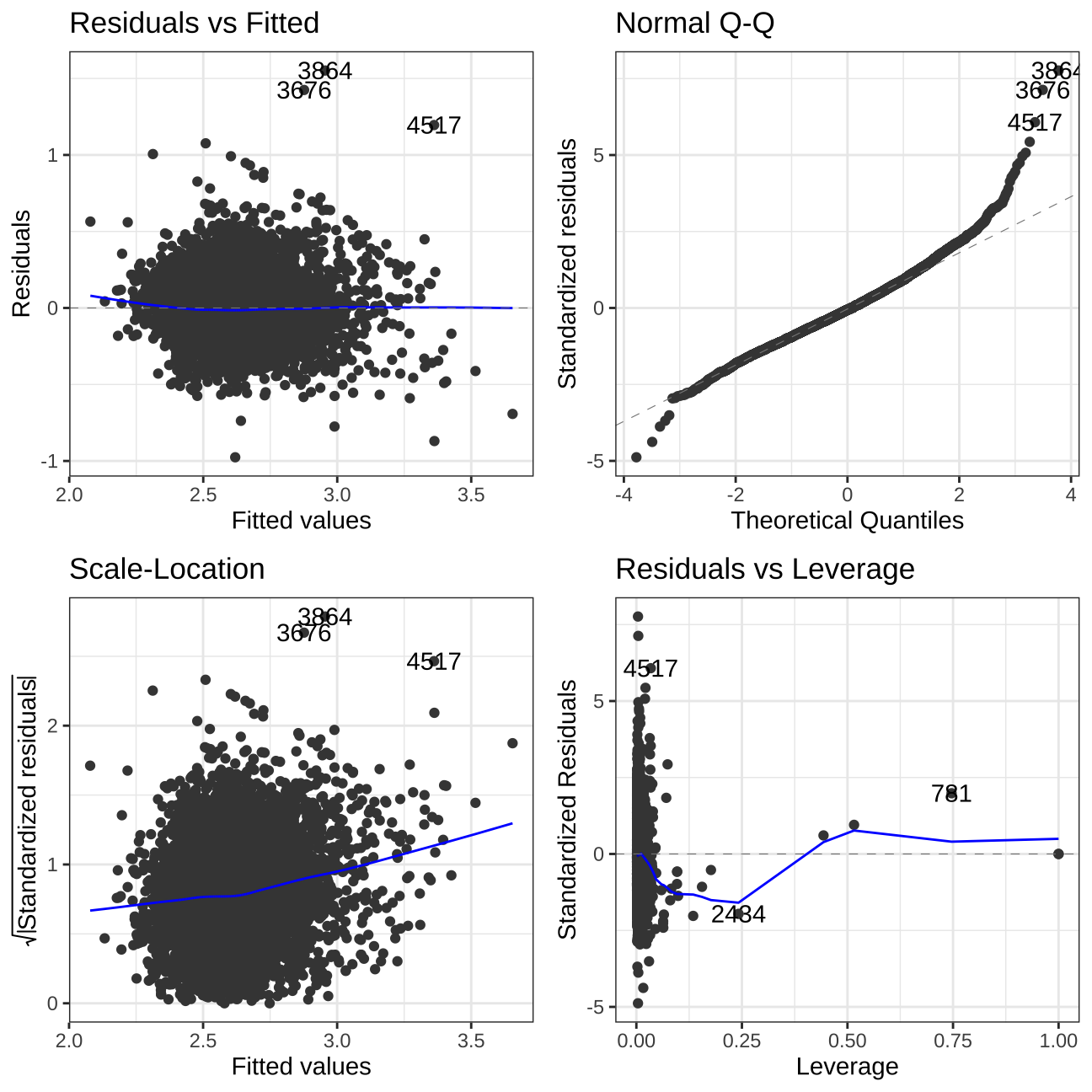
# comparing significance of variables among model iterations
huxreg(model2,
       model3,
       model6,
       model7,
model_wild_west)| (1) | (2) | (3) | (4) | (5) | |
|---|---|---|---|---|---|
| (Intercept) | 6.150 *** | 5.573 *** | 5.715 *** | 5.682 *** | 2.357 *** |
| (0.079) | (0.026) | (0.027) | (0.028) | (0.052) | |
| prop_type_simplifiedCondominium | 0.103 * | 0.072 | 0.061 | 0.050 | 0.017 |
| (0.042) | (0.038) | (0.037) | (0.037) | (0.015) | |
| prop_type_simplifiedHouse | 0.035 | -0.111 ** | -0.054 | -0.062 | -0.028 |
| (0.039) | (0.036) | (0.036) | (0.035) | (0.015) | |
| prop_type_simplifiedLoft | 0.215 *** | 0.116 * | 0.113 * | 0.111 * | 0.044 * |
| (0.057) | (0.052) | (0.051) | (0.050) | (0.021) | |
| prop_type_simplifiedOther | 0.119 ** | 0.001 | 0.002 | 0.016 | 0.014 |
| (0.036) | (0.034) | (0.033) | (0.033) | (0.014) | |
| number_of_reviews | -0.001 *** | -0.002 *** | -0.002 *** | -0.002 *** | -0.001 *** |
| (0.000) | (0.000) | (0.000) | (0.000) | (0.000) | |
| review_scores_rating | 0.000 | ||||
| (0.001) | |||||
| room_typeHotel room | 0.297 ** | 0.540 *** | 0.497 *** | 0.509 *** | 0.278 *** |
| (0.102) | (0.093) | (0.091) | (0.091) | (0.064) | |
| room_typePrivate room | -0.376 *** | -0.249 *** | -0.234 *** | -0.228 *** | -0.001 |
| (0.015) | (0.014) | (0.014) | (0.014) | (0.011) | |
| room_typeShared room | -0.252 *** | -0.297 *** | -0.285 *** | -0.297 *** | -0.144 *** |
| (0.063) | (0.058) | (0.057) | (0.056) | (0.023) | |
| bathrooms | 0.124 *** | 0.118 *** | 0.114 *** | 0.048 *** | |
| (0.023) | (0.023) | (0.023) | (0.009) | ||
| bedrooms | 0.048 *** | 0.039 ** | 0.042 *** | 0.053 *** | |
| (0.013) | (0.012) | (0.012) | (0.005) | ||
| beds | -0.025 ** | ||||
| (0.008) | |||||
| accommodates | 0.148 *** | 0.138 *** | 0.131 *** | 0.050 *** | |
| (0.007) | (0.006) | (0.006) | (0.002) | ||
| regionzone_2 | -0.139 *** | -0.134 *** | -0.059 *** | ||
| (0.017) | (0.017) | (0.007) | |||
| regionzone_3 | -0.196 *** | -0.187 *** | -0.079 *** | ||
| (0.018) | (0.018) | (0.007) | |||
| regionzone_4 | -0.199 *** | -0.192 *** | -0.082 *** | ||
| (0.022) | (0.022) | (0.009) | |||
| regionzone_5 | -0.335 *** | -0.325 *** | -0.130 *** | ||
| (0.020) | (0.020) | (0.008) | |||
| cancellation_policymoderate | 0.008 | 0.009 | |||
| (0.015) | (0.006) | ||||
| cancellation_policystrict_14_with_grace_period | 0.143 *** | 0.049 *** | |||
| (0.016) | (0.007) | ||||
| cancellation_policysuper_strict_30 | 0.132 | -0.046 | |||
| (0.492) | (0.201) | ||||
| cancellation_policysuper_strict_60 | 0.027 | -0.067 | |||
| (0.491) | (0.201) | ||||
| reviews_per_month | -0.048 *** | ||||
| (0.004) | |||||
| review_scores_value | -0.046 *** | ||||
| (0.003) | |||||
| review_scores_cleanliness | 0.021 *** | ||||
| (0.003) | |||||
| review_scores_checkin | 0.012 ** | ||||
| (0.004) | |||||
| review_scores_location | 0.021 *** | ||||
| (0.004) | |||||
| security_deposit | 0.000 *** | ||||
| (0.000) | |||||
| rating_groupUnder 90 | -0.033 *** | ||||
| (0.009) | |||||
| instant_bookableTRUE | 0.038 *** | ||||
| (0.006) | |||||
| availability_365 | 0.000 *** | ||||
| (0.000) | |||||
| availability_90 | 0.001 *** | ||||
| (0.000) | |||||
| maximum_nights | 0.000 * | ||||
| (0.000) | |||||
| minimum_nights | -0.016 *** | ||||
| (0.003) | |||||
| is_elevatorTRUE | 0.011 * | ||||
| (0.005) | |||||
| is_shampooTRUE | 0.011 * | ||||
| (0.005) | |||||
| number_of_reviews:reviews_per_month | 0.000 *** | ||||
| (0.000) | |||||
| room_typeHotel room:bedrooms | -0.104 * | ||||
| (0.048) | |||||
| room_typePrivate room:bedrooms | -0.103 *** | ||||
| (0.008) | |||||
| room_typeShared room:bedrooms | |||||
| N | 6285 | 6285 | 6285 | 6285 | 6285 |
| R2 | 0.115 | 0.263 | 0.297 | 0.308 | 0.391 |
| logLik | -5206.674 | -4633.202 | -4484.509 | -4432.369 | 1207.271 |
| AIC | 10435.349 | 9294.405 | 9003.017 | 8906.737 | -2338.542 |
| *** p < 0.001; ** p < 0.01; * p < 0.05. | |||||
The residuals behave in an appropriate way, hence I assume that the model is correct. Though there is a slight gradient in Scale-Location, and slight tendency in Residuals vs Fitted. The Leverage tends around the mean and the normal Q-Q is linear for the most part. These slight issues are due to the quality of the data scraper.
From the table comparing all the models I can spot, that our R-squared went up through out the process of finding the best solution. I can as well spot which variables were added and dropped at which stages.
Model applyinh and predicting the outcome
Now, I will find a price of the Airbnbs that are apartment with a private room, have at least 10 reviews, and an average rating of at least 90.
I am using the logarithmic model log(total_price_4_days) in the predict function since my regression is based on the log(total_price_4_days). First, I will create a new table that I will filter according to the conditions above. In the next step, I will anti-log the model_wild_west. At the end, I will predict the prices for my filtered accommodations and I will create for them the Confidence Intervals. I will do it in two ways in order to compare our scores.
munich_listings_predict<- munich_listings_region %>%
  mutate(price=log(total_price_4_days)) %>% #converting to log form for prediction
  filter(room_type=="Private room" &
           number_of_reviews>=10 &
           rating_group=="Over 90")


predict_df<-10^predict(model_wild_west, # converting from log form to nominal
                    newdata = munich_listings_predict,
                    interval= "confidence")
#sanity check
summary(predict_df)
## fit lwr upr
## Min. :136 Min. :116 Min. :157
## 1st Qu.:256 1st Qu.:242 1st Qu.:271
## Median :300 Median :282 Median :316
## Mean :315 Mean :296 Mean :336
## 3rd Qu.:358 3rd Qu.:338 3rd Qu.:377
## Max. :762 Max. :649 Max. :958#using broom augment
model_prediction <- broom::augment(model_wild_west,
newdata= munich_listings_predict)
model_prediction <- model_prediction %>%
mutate(lower_95=10^.fitted-1.96*abs(10^(.resid)),#creating 95% confidence interval
upper_95=10^.fitted+1.96*abs(10^(.resid))) %>%
select(.fitted,
lower_95,
upper_95,
total_price_4_days) %>%
mutate(.fitted=10^.fitted)
#sanity check
summary(model_prediction)## .fitted lower_95 upper_95 total_price_4_days
## Min. :136 Min. :134 Min. :138 Min. : 92
## 1st Qu.:256 1st Qu.:254 1st Qu.:258 1st Qu.: 217
## Median :300 Median :297 Median :302 Median : 280
## Mean :315 Mean :313 Mean :317 Mean : 327
## 3rd Qu.:358 3rd Qu.:356 3rd Qu.:359 3rd Qu.: 380
## Max. :762 Max. :762 Max. :763 Max. :4036Using the predict and augment function I can observe a mean price of around 315, which is close to the actual total mean price of 327. I also see that the 1st and 3rd quartiles for both of the prediction methods all line up. Differences appear in the lower and upper confidence level boundaries between the two functions, where the predict function’s interval actually captures the true mean, the augment misses it by €10. Despite this I can get a sense of confidence for the linear regression’s accuracy due to the tight spread and capturing of the true mean. The next step is conducting a sanity check by checking the RMSE of my model.
Data Training and RMSE
In the next step I will split my data into two parts. I will train one part and later test another one. In the next step I will compare the results.
set.seed(1234)
train_test_split <- initial_split(munich_listings_predict, prop=0.7) # splitting dataset
munich_train<- training(train_test_split)
munich_test<- testing(train_test_split)

rmse_train <- munich_train %>%  #training portion for RMSE
  mutate(predictions=predict(model_wild_west,.)) %>%
  summarise(sqrt(sum(predictions-log(total_price_4_days))**2/n())) %>%
  pull()
rmse_train
## [1] 82.7rmse_test <- munich_test %>%
mutate(predictions=predict(model_wild_west,.)) %>%
summarise(sqrt(sum(predictions-log(total_price_4_days))**2/n())) %>%
pull()
rmse_test## [1] 54.1I can see that the RMSE is an order of magnitude below our prices, which confirms that though our R^2 is low, the accuracy is very high.
Thank you for your interest in our study project. I hope you found it interesting.
