Predicting interest rates using K-fold CV,LASSO & OLS regression

In this piece I will analyse the data on interest rates in the Lendign Club. First I will conduct the ICE of the data together with visualisation of the variables disributions and correlations for better understanding. Then, I will first build a linear regression model, then such techniques oa out of sample testing, k-fold cross validation. I will also conduct regularisation using LASSO regression and compare the scores to the OLS method. Later, I will improve my model by adding time variables, yeld bond variables, CPI index.

Load and prepare the data

I start by loading the data to R in a dataframe.

lc_raw <- read_csv("~/Documents/LBS/Data Science/Session 03/LendingClub Data.csv",  skip=1) %>%  clean_names() # use janitor::clean_names()

ICE the data: Inspect, Clean, Explore

Any data science engagement starts with ICE. Inspect, Clean and Explore the data.

#glimpse(lc_raw) 

lc_clean<- lc_raw %>%
  dplyr::select(-x20:-x80) %>% #delete empty columns
  filter(!is.na(int_rate)) %>%   #delete empty rows
  mutate(
    issue_d = mdy(issue_d),  # lubridate::mdy() to fix date format
    term = factor(term_months),     # turn 'term' into a categorical variable
    delinq_2yrs = factor(delinq_2yrs) # turn 'delinq_2yrs' into a categorical variable
  ) %>% 
  dplyr::select(-emp_title,-installment, -term_months, everything()) %>% mutate(emp_length=as.factor(emp_length)) #move some not-so-important variables to the end. 


#glimpse(lc_clean) 
summary(lc_clean)

##     int_rate      loan_amnt          dti         delinq_2yrs   
##  Min.   :0.05   Min.   :  500   Min.   : 0.00   0      :33782  
##  1st Qu.:0.09   1st Qu.: 5500   1st Qu.: 8.14   1      : 3141  
##  Median :0.12   Median :10000   Median :13.36   2      :  637  
##  Mean   :0.12   Mean   :11253   Mean   :13.28   3      :  213  
##  3rd Qu.:0.15   3rd Qu.:15000   3rd Qu.:18.58   4      :   56  
##  Max.   :0.25   Max.   :35000   Max.   :29.99   5      :   22  
##                                                 (Other):   18  
##    annual_inc         grade               emp_length    home_ownership    
##  Min.   :   4000   Length:37869       10+ years: 8405   Length:37869      
##  1st Qu.:  40800   Class :character   < 1 year : 4384   Class :character  
##  Median :  59534   Mode  :character   2 years  : 4168   Mode  :character  
##  Mean   :  69148                      3 years  : 3910                     
##  3rd Qu.:  82800                      4 years  : 3305                     
##  Max.   :6000000                      5 years  : 3146                     
##                                       (Other)  :10551                     
##  verification_status    issue_d             zip_code          addr_state       
##  Length:37869        Min.   :2007-06-01   Length:37869       Length:37869      
##  Class :character    1st Qu.:2010-05-01   Class :character   Class :character  
##  Mode  :character    Median :2011-02-01   Mode  :character   Mode  :character  
##                      Mean   :2010-11-05                                        
##                      3rd Qu.:2011-08-01                                        
##                      Max.   :2011-12-01                                        
##                                                                                
##  loan_status            desc             purpose             title          
##  Length:37869       Length:37869       Length:37869       Length:37869      
##  Class :character   Class :character   Class :character   Class :character  
##  Mode  :character   Mode  :character   Mode  :character   Mode  :character  
##                                                                             
##                                                                             
##                                                                             
##                                                                             
##  term        term_months    installment    emp_title        
##  36:27674   Min.   :36.0   Min.   :  16   Length:37869      
##  60:10195   1st Qu.:36.0   1st Qu.: 169   Class :character  
##             Median :36.0   Median : 288   Mode  :character  
##             Mean   :42.5   Mean   : 333                     
##             3rd Qu.:60.0   3rd Qu.: 449                     
##             Max.   :60.0   Max.   :1305                     
##

The data is now in a clean format stored in the dataframe “lc_clean.”

Explore the data by building some visualizations.

# Build a histogram of interest rates.
ggplot(lc_clean, aes(x=int_rate))+ 
  geom_histogram(bins=20) + 
  labs(title="Histogram of Interest Rate",
       x="Interest Rate",
       y="Count")+
  scale_x_continuous(labels = scales::percent)+
  theme_bw()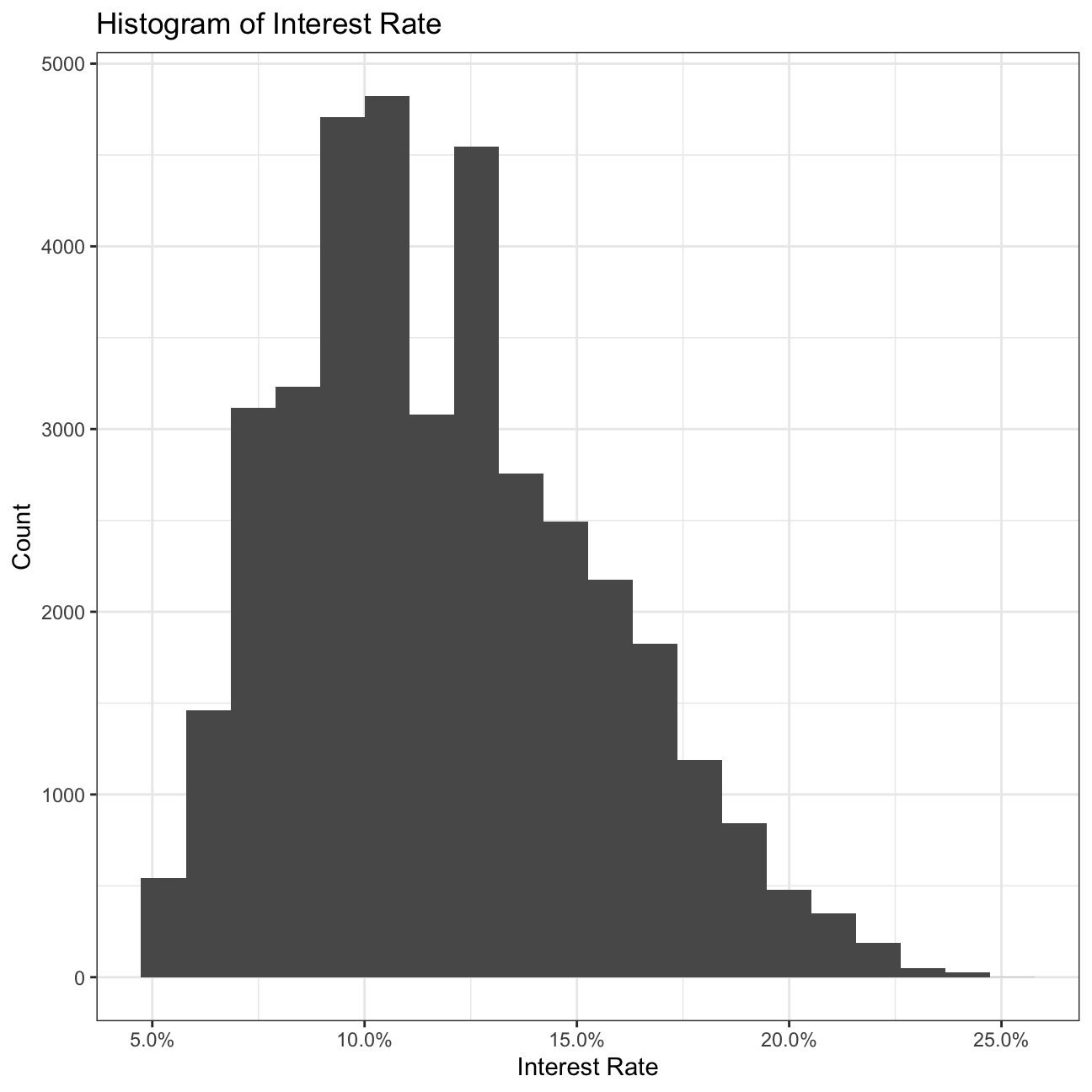

# Build a histogram of interest rates with different color for loans of different grades 
ggplot(lc_clean, aes(x=int_rate, fill=grade))+ 
  geom_histogram(bins=20)+
  labs(title="Histogram of Interest Rate by Grade",
       x="Interest Rate",
       y="Count")+
  scale_x_continuous(labels = scales::percent)+
  theme_bw()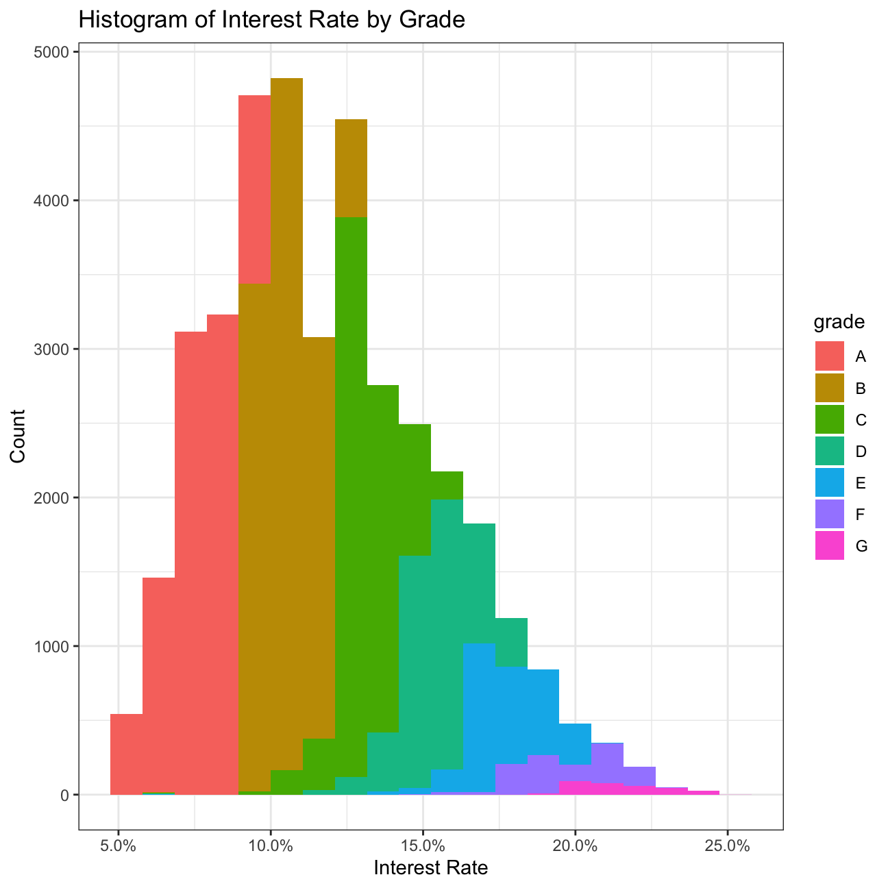

# a scatter plot of loan amount against interest rate with the line of best fit
ggplot(lc_clean[seq(1, nrow(lc_clean), 10), ] , aes(y=int_rate, x=loan_amnt)) +  geom_smooth(method="lm",se=0)+
  geom_point()+
scale_x_continuous(label=scales::dollar)+
  labs(y="Interest Rate", x="Annual Income")+
  theme_bw()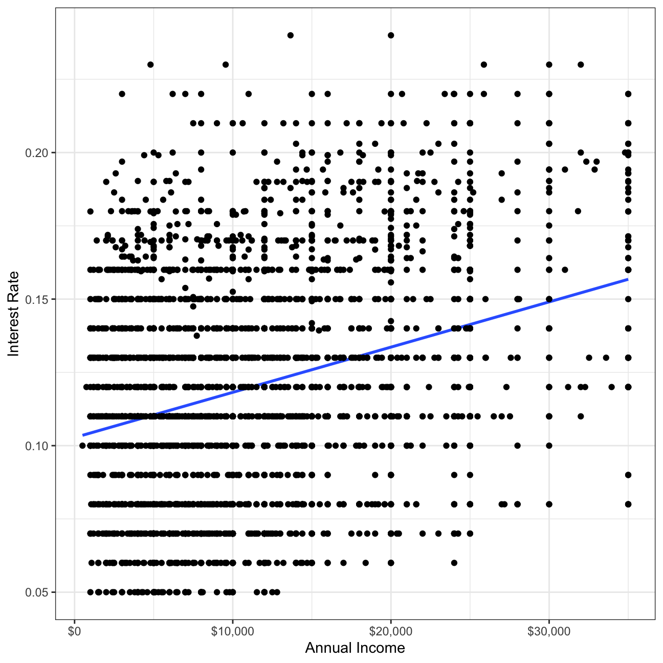

# a scatter plot of annual income against interest rate and with the line of best fit 
ggplot(lc_clean[seq(1, nrow(lc_clean), 10), ] , aes(y=int_rate, x=annual_inc)) + 
  geom_point(size=0.1)+ 
  geom_smooth(method="lm", se=0) +
  scale_x_continuous(label=scales::dollar)+
  labs(y="Interest Rate", x="Annual Income")+
  theme_bw()

# box plots of the interest rate for every value of delinquencies
ggplot(lc_clean , aes(y=int_rate, x=delinq_2yrs, colour= delinq_2yrs)) + 
  geom_boxplot()+
  # geom_jitter()+
  theme_bw()+
   scale_y_continuous(labels=scales::percent)+
  theme(legend.position = "none")+
  labs(
    title = "Do delinquencies in the last two years impact interest rate charged?",
    x= "Number of delinquecies in last two years", y="Interest Rate"
  )+
  theme_bw()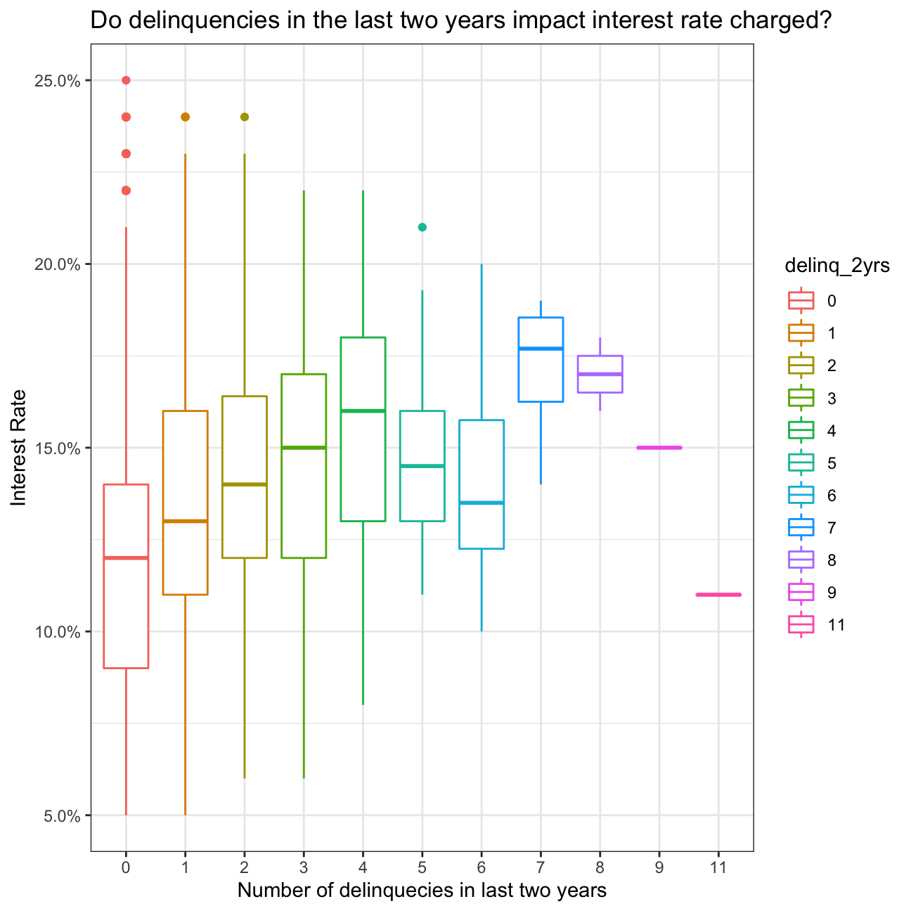

#loan period vs interest rate
ggplot(lc_clean, aes(x=term, y = int_rate))+
  geom_boxplot()+
  labs(title="Interest Rate Spread by Loan Term",
       x="Loan Term in Months",
       y="Interest Rate")+
  scale_y_continuous(labels=scales::percent)+
  theme_bw()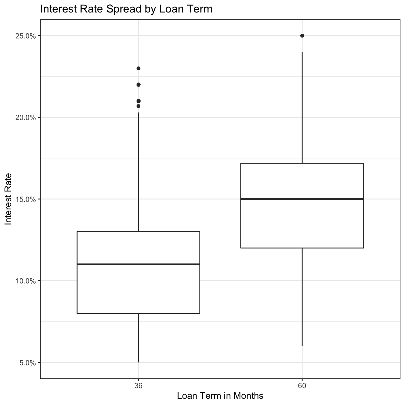

#home ownership vs interest rate
ggplot(lc_clean, aes(x=home_ownership, y = int_rate))+
  geom_boxplot()+
  labs(title="Interest Rate Spread by Ownership Status",
       x="Ownership Status",
       y="Interest Rate")+
  scale_y_continuous(labels=scales::percent)+
  theme_bw()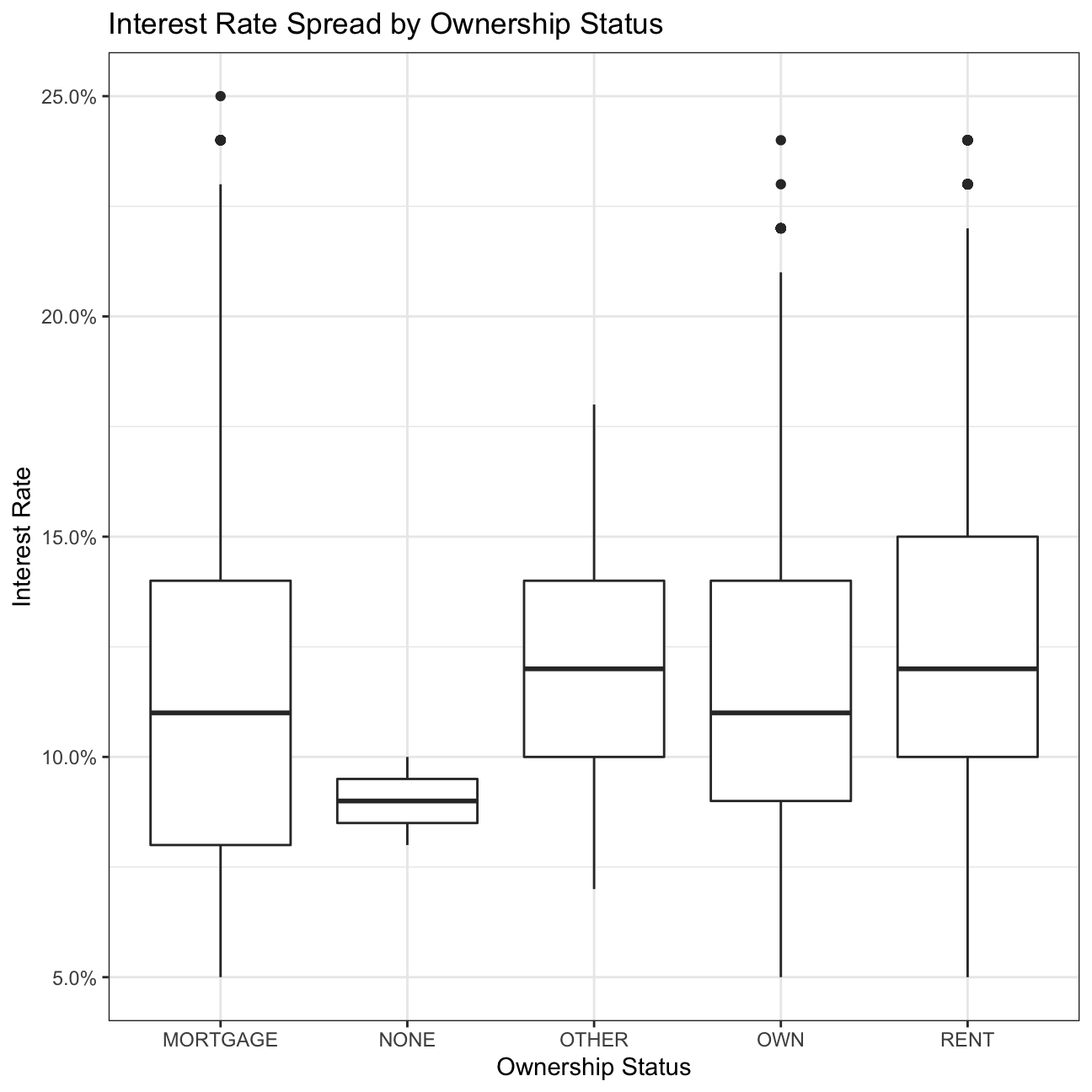

#Employment Length vs Interest 
ggplot(lc_clean, aes(x=emp_length, y = int_rate))+
  geom_boxplot()+
  labs(title="Interest Rate Spread by Ownership Status",
       x="Ownership Status",
       y="Interest Rate")+
  scale_y_continuous(labels=scales::percent)+
  theme_bw()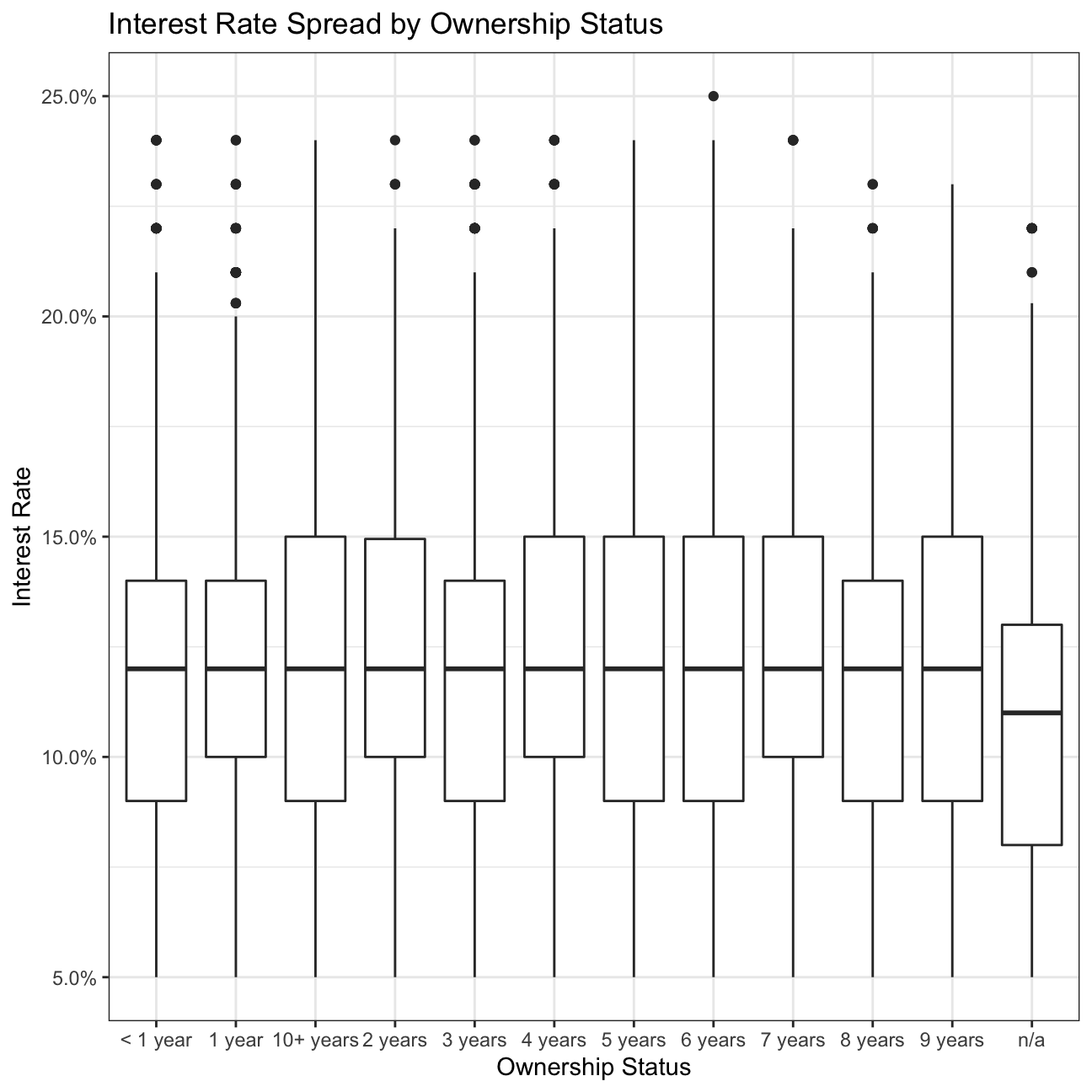

Estimatimation of simple linear regression models

I start with a simple but quite powerful model.

#I will use the lm command to estimate a regression model with the following variables "loan_amnt",  "term", "dti", "annual_inc", and "grade"

model1<-lm( int_rate ~ loan_amnt+ term+ dti+ annual_inc+ grade, data = lc_clean
  )
summary(model1) # noticed that annual income has a p value of over 0.05

## 
## Call:
## lm(formula = int_rate ~ loan_amnt + term + dti + annual_inc + 
##     grade, data = lc_clean)
## 
## Residuals:
##      Min       1Q   Median       3Q      Max 
## -0.11883 -0.00704 -0.00034  0.00683  0.03508 
## 
## Coefficients:
##              Estimate Std. Error t value Pr(>|t|)    
## (Intercept)  7.17e-02   1.69e-04  424.36  < 2e-16 ***
## loan_amnt    1.48e-07   8.28e-09   17.81  < 2e-16 ***
## term60       3.61e-03   1.42e-04   25.43  < 2e-16 ***
## dti          4.33e-05   8.27e-06    5.23  1.7e-07 ***
## annual_inc  -9.73e-10   9.28e-10   -1.05     0.29    
## gradeB       3.55e-02   1.49e-04  238.25  < 2e-16 ***
## gradeC       6.02e-02   1.66e-04  362.78  < 2e-16 ***
## gradeD       8.17e-02   1.91e-04  428.75  < 2e-16 ***
## gradeE       1.00e-01   2.48e-04  402.66  < 2e-16 ***
## gradeF       1.20e-01   3.67e-04  325.41  < 2e-16 ***
## gradeG       1.35e-01   6.21e-04  218.24  < 2e-16 ***
## ---
## Signif. codes:  0 '***' 0.001 '**' 0.01 '*' 0.05 '.' 0.1 ' ' 1
## 
## Residual standard error: 0.0106 on 37858 degrees of freedom
## Multiple R-squared:  0.92,   Adjusted R-squared:  0.92 
## F-statistic: 4.34e+04 on 10 and 37858 DF,  p-value: <2e-16

Questions on the model

a. Are all variables statistically significant?

I noticed that in model1 annual_inc is the only insignificant variable. Therefore, it will be reasonable to exclude it in my future models.

b. How to interpret the coefficient of the Term60 dummy variable? Of the grade B dummy variable?

All things being equal and on average compared to term 30, the interest rate increases by 3.608e-03 percentage point if the lending time amounts to 60 (term is equal to 60).
All things being equal and on average compared to grade A, the interest rate increases by 3.554e-02 percentage point if the grade of user is B category.

c. How much explanatory power does the model have? My model has 91.97% explanatory power (I checked it looking at Adjusted R-squared).

d. Approximately, how wide would the 95% confidence interval of any prediction based on this model be? The 95% Confidence Interval of any prediction based on model1, would amount to 1.96*0.01056 = ~±0.021.

Feature Engineering

Let’s build progressively more complex models with more features.

I will add to the previous model an interaction between loan amount and grade. The "var1*var2" notation is used to define an interaction term in the linear regression model. This will add the interaction and the individual variables to the model.

model2 <-lm( int_rate ~ loan_amnt*grade+ term+ dti+ annual_inc, data = lc_clean
  )

summary(model2)

## 
## Call:
## lm(formula = int_rate ~ loan_amnt * grade + term + dti + annual_inc, 
##     data = lc_clean)
## 
## Residuals:
##      Min       1Q   Median       3Q      Max 
## -0.11981 -0.00723 -0.00006  0.00659  0.03746 
## 
## Coefficients:
##                   Estimate Std. Error t value Pr(>|t|)    
## (Intercept)       7.17e-02   2.35e-04  305.76  < 2e-16 ***
## loan_amnt         1.53e-07   2.03e-08    7.54  4.9e-14 ***
## gradeB            3.62e-02   2.73e-04  132.62  < 2e-16 ***
## gradeC            6.20e-02   2.99e-04  207.45  < 2e-16 ***
## gradeD            8.08e-02   3.48e-04  232.03  < 2e-16 ***
## gradeE            9.63e-02   4.62e-04  208.29  < 2e-16 ***
## gradeF            1.14e-01   7.74e-04  147.70  < 2e-16 ***
## gradeG            1.33e-01   1.55e-03   85.58  < 2e-16 ***
## term60            3.79e-03   1.42e-04   26.64  < 2e-16 ***
## dti               3.84e-05   8.25e-06    4.65  3.3e-06 ***
## annual_inc       -1.22e-09   9.25e-10   -1.32   0.1856    
## loan_amnt:gradeB -6.62e-08   2.44e-08   -2.71   0.0067 ** 
## loan_amnt:gradeC -1.70e-07   2.62e-08   -6.50  8.1e-11 ***
## loan_amnt:gradeD  6.70e-08   2.80e-08    2.40   0.0166 *  
## loan_amnt:gradeE  2.21e-07   3.02e-08    7.32  2.5e-13 ***
## loan_amnt:gradeF  2.78e-07   4.14e-08    6.72  1.8e-11 ***
## loan_amnt:gradeG  1.27e-07   7.26e-08    1.74   0.0814 .  
## ---
## Signif. codes:  0 '***' 0.001 '**' 0.01 '*' 0.05 '.' 0.1 ' ' 1
## 
## Residual standard error: 0.0105 on 37852 degrees of freedom
## Multiple R-squared:  0.92,   Adjusted R-squared:  0.92 
## F-statistic: 2.74e+04 on 16 and 37852 DF,  p-value: <2e-16

I will add to the model the square and the cube of annual income. To do it, I will use the poly(var_name,3) command as a variable in the linear regression model.

model3 <- lm( int_rate ~ loan_amnt*grade+ term+ dti+poly(annual_inc,3), data = lc_clean
  ) 
summary(model3) # makes no difference

## 
## Call:
## lm(formula = int_rate ~ loan_amnt * grade + term + dti + poly(annual_inc, 
##     3), data = lc_clean)
## 
## Residuals:
##      Min       1Q   Median       3Q      Max 
## -0.11981 -0.00724 -0.00006  0.00659  0.03747 
## 
## Coefficients:
##                       Estimate Std. Error t value Pr(>|t|)    
## (Intercept)           7.16e-02   2.28e-04  314.20  < 2e-16 ***
## loan_amnt             1.56e-07   2.05e-08    7.60  3.0e-14 ***
## gradeB                3.62e-02   2.73e-04  132.61  < 2e-16 ***
## gradeC                6.20e-02   2.99e-04  207.40  < 2e-16 ***
## gradeD                8.08e-02   3.48e-04  232.00  < 2e-16 ***
## gradeE                9.63e-02   4.62e-04  208.28  < 2e-16 ***
## gradeF                1.14e-01   7.74e-04  147.70  < 2e-16 ***
## gradeG                1.33e-01   1.55e-03   85.57  < 2e-16 ***
## term60                3.79e-03   1.43e-04   26.55  < 2e-16 ***
## dti                   3.76e-05   8.29e-06    4.53  5.8e-06 ***
## poly(annual_inc, 3)1 -1.59e-02   1.12e-02   -1.42   0.1549    
## poly(annual_inc, 3)2  6.30e-03   1.09e-02    0.58   0.5621    
## poly(annual_inc, 3)3 -8.98e-03   1.08e-02   -0.83   0.4076    
## loan_amnt:gradeB     -6.63e-08   2.44e-08   -2.72   0.0066 ** 
## loan_amnt:gradeC     -1.70e-07   2.62e-08   -6.50  8.2e-11 ***
## loan_amnt:gradeD      6.71e-08   2.80e-08    2.40   0.0165 *  
## loan_amnt:gradeE      2.21e-07   3.02e-08    7.32  2.4e-13 ***
## loan_amnt:gradeF      2.78e-07   4.14e-08    6.72  1.8e-11 ***
## loan_amnt:gradeG      1.27e-07   7.26e-08    1.75   0.0801 .  
## ---
## Signif. codes:  0 '***' 0.001 '**' 0.01 '*' 0.05 '.' 0.1 ' ' 1
## 
## Residual standard error: 0.0105 on 37850 degrees of freedom
## Multiple R-squared:  0.92,   Adjusted R-squared:  0.92 
## F-statistic: 2.43e+04 on 18 and 37850 DF,  p-value: <2e-16

Continuing with the previous model, instead of annual income as a continuous variable, I will break it down into quartiles and use quartile dummy variables.

lc_clean2 <- lc_clean %>% 
  mutate(quartiles_annual_inc = as.factor(ntile(annual_inc, 4)))

model4 <-lm( int_rate ~ loan_amnt*grade+ term+ dti+quartiles_annual_inc, data = lc_clean2
  ) 
summary(model4)  # still makes no difference

## 
## Call:
## lm(formula = int_rate ~ loan_amnt * grade + term + dti + quartiles_annual_inc, 
##     data = lc_clean2)
## 
## Residuals:
##      Min       1Q   Median       3Q      Max 
## -0.11977 -0.00720 -0.00006  0.00660  0.03758 
## 
## Coefficients:
##                        Estimate Std. Error t value Pr(>|t|)    
## (Intercept)            7.19e-02   2.41e-04  297.70  < 2e-16 ***
## loan_amnt              1.62e-07   2.05e-08    7.89  3.1e-15 ***
## gradeB                 3.62e-02   2.73e-04  132.52  < 2e-16 ***
## gradeC                 6.20e-02   2.99e-04  207.27  < 2e-16 ***
## gradeD                 8.08e-02   3.48e-04  231.88  < 2e-16 ***
## gradeE                 9.63e-02   4.62e-04  208.27  < 2e-16 ***
## gradeF                 1.14e-01   7.73e-04  147.72  < 2e-16 ***
## gradeG                 1.33e-01   1.55e-03   85.57  < 2e-16 ***
## term60                 3.78e-03   1.42e-04   26.53  < 2e-16 ***
## dti                    3.67e-05   8.26e-06    4.45  8.8e-06 ***
## quartiles_annual_inc2 -2.62e-04   1.55e-04   -1.69   0.0907 .  
## quartiles_annual_inc3 -3.99e-04   1.59e-04   -2.51   0.0121 *  
## quartiles_annual_inc4 -5.38e-04   1.69e-04   -3.18   0.0015 ** 
## loan_amnt:gradeB      -6.64e-08   2.44e-08   -2.72   0.0066 ** 
## loan_amnt:gradeC      -1.70e-07   2.62e-08   -6.48  9.1e-11 ***
## loan_amnt:gradeD       6.77e-08   2.80e-08    2.42   0.0156 *  
## loan_amnt:gradeE       2.20e-07   3.02e-08    7.30  2.9e-13 ***
## loan_amnt:gradeF       2.77e-07   4.14e-08    6.69  2.3e-11 ***
## loan_amnt:gradeG       1.27e-07   7.26e-08    1.75   0.0809 .  
## ---
## Signif. codes:  0 '***' 0.001 '**' 0.01 '*' 0.05 '.' 0.1 ' ' 1
## 
## Residual standard error: 0.0105 on 37850 degrees of freedom
## Multiple R-squared:  0.92,   Adjusted R-squared:  0.92 
## F-statistic: 2.43e+04 on 18 and 37850 DF,  p-value: <2e-16

I will compare now the performance of these four models using the anova command

anova(model1, model2, model3, model4
      )

Res.Df	RSS	Df	Sum of Sq	F	Pr(>F)
3.79e+04	4.22
3.79e+04	4.19	6	0.0332	50	1.64e-61
3.78e+04	4.19	2	0.000107	0.484	0.616
3.78e+04	4.19	0	0.000915

Conclusions

a. Which of the four models has the most explanatory power in sample Models 2, 3 & 4 have the most explanatory power amounting to 0.9204. (The Adjusted R-squared is the same for all the 3 models)

b. In model 2, how to interpret the estimated coefficient of the interaction term between grade B and loan amount? All things being equal and on average compared to grade A, if the loan amount increase by 10 000, the interest rate for grade B useres will decrease by 6.617e-04 percentage point.

c. The problem of multicolinearity describes the situations where one feature is highly correlated with other fueatures (or with a linear combination of other features). If the goal is to use the model to make predictions, should you be concerned by the problem of multicolinearity? Why, or why not? Multicolinearity impacts inference more than prediction, so for the case of prediction it is not very relevant. However, if one is using the model to explain their existing dataset they may have inaccurate results.

Out of sample testing

Let’s check the predictive accuracy of model2 by holding out a subset of the data to use as testing. This method is sometimes refered to as the hold-out method for out-of-sample testing.

#split the data in dataframe called "testing" and another one called  "training". The "training" dataframe should have 80% of the data and the "testing" dataframe 20%.
set.seed(176823769)
train_test_split <- initial_split(lc_clean2, prop=0.8) # splitting dataset
lc_clean_train<- training(train_test_split)
lc_clean_test<- testing(train_test_split) 


#Fit model2 on the training set 
model2_training<-lm(int_rate ~ loan_amnt + term+ dti + annual_inc + grade +grade:loan_amnt, data=lc_clean_train)
summary(model2_training)

## 
## Call:
## lm(formula = int_rate ~ loan_amnt + term + dti + annual_inc + 
##     grade + grade:loan_amnt, data = lc_clean_train)
## 
## Residuals:
##      Min       1Q   Median       3Q      Max 
## -0.11977 -0.00721 -0.00004  0.00659  0.03764 
## 
## Coefficients:
##                   Estimate Std. Error t value Pr(>|t|)    
## (Intercept)       7.16e-02   2.64e-04  271.57  < 2e-16 ***
## loan_amnt         1.59e-07   2.25e-08    7.05  1.9e-12 ***
## term60            3.77e-03   1.59e-04   23.69  < 2e-16 ***
## dti               4.07e-05   9.23e-06    4.41  1.1e-05 ***
## annual_inc       -8.11e-10   1.19e-09   -0.68    0.497    
## gradeB            3.62e-02   3.04e-04  119.16  < 2e-16 ***
## gradeC            6.20e-02   3.33e-04  186.19  < 2e-16 ***
## gradeD            8.09e-02   3.87e-04  209.01  < 2e-16 ***
## gradeE            9.60e-02   5.15e-04  186.64  < 2e-16 ***
## gradeF            1.14e-01   8.72e-04  130.70  < 2e-16 ***
## gradeG            1.34e-01   1.75e-03   76.57  < 2e-16 ***
## loan_amnt:gradeB -7.33e-08   2.72e-08   -2.70    0.007 ** 
## loan_amnt:gradeC -1.75e-07   2.92e-08   -6.00  2.0e-09 ***
## loan_amnt:gradeD  6.79e-08   3.11e-08    2.18    0.029 *  
## loan_amnt:gradeE  2.29e-07   3.35e-08    6.85  7.5e-12 ***
## loan_amnt:gradeF  2.97e-07   4.62e-08    6.44  1.2e-10 ***
## loan_amnt:gradeG  7.97e-08   8.21e-08    0.97    0.331    
## ---
## Signif. codes:  0 '***' 0.001 '**' 0.01 '*' 0.05 '.' 0.1 ' ' 1
## 
## Residual standard error: 0.0105 on 30279 degrees of freedom
## Multiple R-squared:  0.921,  Adjusted R-squared:  0.921 
## F-statistic: 2.2e+04 on 16 and 30279 DF,  p-value: <2e-16

#Calculate the RMSE of the model in the training set (in sample)
rmse_training<-sqrt(mean((residuals(model2_training))^2))
#Use the model to make predictions out of sample in the testing set
pred<-predict(model2_training,lc_clean_test)
#Calculate the RMSE of the model in the testing set (out of sample)
rmse_testing<- RMSE(pred,lc_clean_test$int_rate)

rmse_training

## [1] 0.0105

rmse_testing

## [1] 0.0106

The predictive accuracy of model 2 does not much deteriorate when I move from in sample to out of sample testing. For purpose of checking it I compare the rmse_training to rmse_testing (0.0104 compared to 0.01061). I tried to check if the model is sensitive for the multiple random seed choices and I discovered that the model is not much sensitive (rmse is still a factor of e-2). There isn’t any evidence of overfitting.

k-fold cross validation

I can also do out of sample testing using the method of k-fold cross validation. Using the caret package this is easy.

#the method "cv" stands for cross validation. I am going to create 10 folds.  

control <- trainControl (
    method="cv",
    number=10,
    verboseIter=TRUE) #by setting this to true the model will report its progress after each estimation

#train the model and report the results using k-fold cross validation
plsFit<-train(
    int_rate ~ loan_amnt + term+ dti + annual_inc + grade +grade:loan_amnt ,
    lc_clean,
   method = "lm",
    trControl = control
   )

## + Fold01: intercept=TRUE 
## - Fold01: intercept=TRUE 
## + Fold02: intercept=TRUE 
## - Fold02: intercept=TRUE 
## + Fold03: intercept=TRUE 
## - Fold03: intercept=TRUE 
## + Fold04: intercept=TRUE 
## - Fold04: intercept=TRUE 
## + Fold05: intercept=TRUE 
## - Fold05: intercept=TRUE 
## + Fold06: intercept=TRUE 
## - Fold06: intercept=TRUE 
## + Fold07: intercept=TRUE 
## - Fold07: intercept=TRUE 
## + Fold08: intercept=TRUE 
## - Fold08: intercept=TRUE 
## + Fold09: intercept=TRUE 
## - Fold09: intercept=TRUE 
## + Fold10: intercept=TRUE 
## - Fold10: intercept=TRUE 
## Aggregating results
## Fitting final model on full training set

summary(plsFit)

## 
## Call:
## lm(formula = .outcome ~ ., data = dat)
## 
## Residuals:
##      Min       1Q   Median       3Q      Max 
## -0.11981 -0.00723 -0.00006  0.00659  0.03746 
## 
## Coefficients:
##                     Estimate Std. Error t value Pr(>|t|)    
## (Intercept)         7.17e-02   2.35e-04  305.76  < 2e-16 ***
## loan_amnt           1.53e-07   2.03e-08    7.54  4.9e-14 ***
## term60              3.79e-03   1.42e-04   26.64  < 2e-16 ***
## dti                 3.84e-05   8.25e-06    4.65  3.3e-06 ***
## annual_inc         -1.22e-09   9.25e-10   -1.32   0.1856    
## gradeB              3.62e-02   2.73e-04  132.62  < 2e-16 ***
## gradeC              6.20e-02   2.99e-04  207.45  < 2e-16 ***
## gradeD              8.08e-02   3.48e-04  232.03  < 2e-16 ***
## gradeE              9.63e-02   4.62e-04  208.29  < 2e-16 ***
## gradeF              1.14e-01   7.74e-04  147.70  < 2e-16 ***
## gradeG              1.33e-01   1.55e-03   85.58  < 2e-16 ***
## `loan_amnt:gradeB` -6.62e-08   2.44e-08   -2.71   0.0067 ** 
## `loan_amnt:gradeC` -1.70e-07   2.62e-08   -6.50  8.1e-11 ***
## `loan_amnt:gradeD`  6.70e-08   2.80e-08    2.40   0.0166 *  
## `loan_amnt:gradeE`  2.21e-07   3.02e-08    7.32  2.5e-13 ***
## `loan_amnt:gradeF`  2.78e-07   4.14e-08    6.72  1.8e-11 ***
## `loan_amnt:gradeG`  1.27e-07   7.26e-08    1.74   0.0814 .  
## ---
## Signif. codes:  0 '***' 0.001 '**' 0.01 '*' 0.05 '.' 0.1 ' ' 1
## 
## Residual standard error: 0.0105 on 37852 degrees of freedom
## Multiple R-squared:  0.92,   Adjusted R-squared:  0.92 
## F-statistic: 2.74e+04 on 16 and 37852 DF,  p-value: <2e-16

Conclusions

The RMSE for both methods is the same, however the k-fold cross validation method gives a range of answers and is more reliable since it checks k times and for k samples. However, the drawback of k-fold cross validation is that it takes much longer time.

Sample size estimation and learning curves

I can use the hold out method for out-of-sample testing to check if the sample is sufficiently large to estimate the model reliably. The idea is to set aside some of the data as a testing set. From the remaining data I will draw progressively larger training sets and check how the performance of the model on the testing set changes. If the performance no longer improves with larger datasets I will be sure that the sample is large enough.

#select a testing dataset (25% of all data)
set.seed(12)

train_test_split <- initial_split(lc_clean, prop = 0.75)
remaining <- training(train_test_split)
testing <- testing(train_test_split)

#run 30 models starting from a tiny training set drawn from the training data and progressively increasing its size. The testing set remains the same in all iterations.

#initiating the model by setting some parameters to zero
rmse_sample <- 0
sample_size<-0
Rsq_sample<-0

for(i in 1:30) {
#from the remaining dataset select a smaller subset to training the data
set.seed(100)
sample

  learning_split <- initial_split(remaining, prop = i/200)
  training <- training(learning_split)
  sample_size[i]=nrow(training)
  
  #traing the model on the small dataset
  model3<-lm(int_rate ~ loan_amnt + term+ dti + annual_inc + grade + grade:loan_amnt, training)
  #test the performance of the model on the large testing dataset. This stays fixed for all iterations.
  pred<-predict(model3,testing)
  rmse_sample[i]<-RMSE(pred,testing$int_rate)
  Rsq_sample[i]<-R2(pred,testing$int_rate)
}
plot(sample_size,rmse_sample)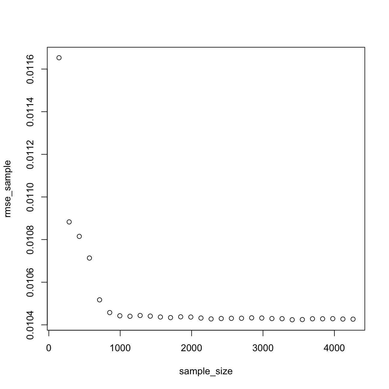

plot(sample_size,Rsq_sample)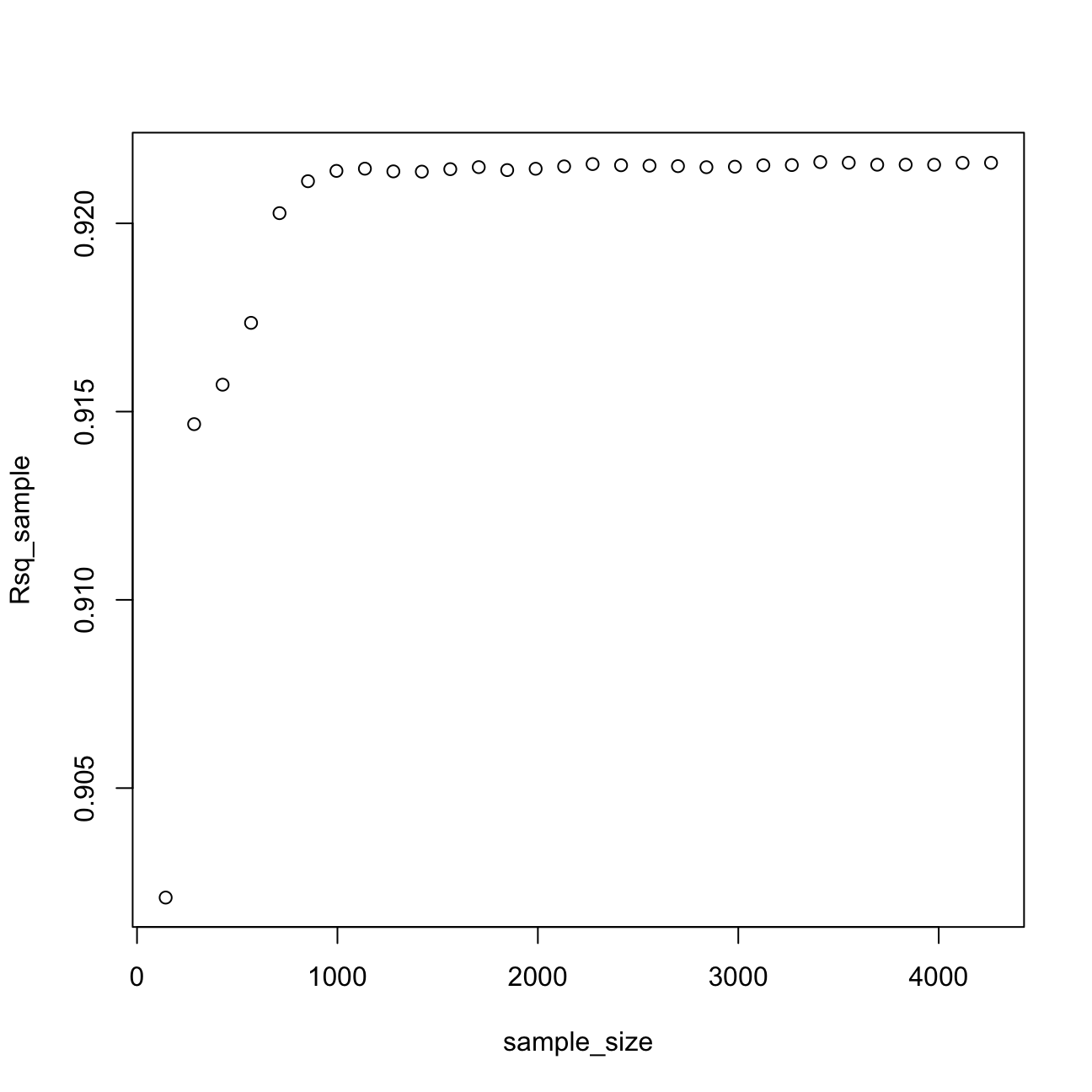

After analysing the graphs above, I noticed that the sample size that would estimate model 3 reliably is 1500. Once I reach this sample size, I can still try to reduce the prediction error by regularization or using the k-fold cross validation method.

Regularization using LASSO regression

If we are in the region of the learning curve where we do not have enough data, one option is to use a regularization method such as LASSO.

Let’s try to estimate large and complicated model (many interactions and polynomials) on a small training dataset using OLS regression and hold-out validation method.

#split the data in testing and training. The training test is really small.
set.seed(1234)
train_test_split <- initial_split(lc_clean, prop = 0.01)
training <- training(train_test_split)
testing <- testing(train_test_split)

model_lm<-lm(int_rate ~ poly(loan_amnt,3) + term+ dti + annual_inc + grade +grade:poly(loan_amnt,3):term +poly(loan_amnt,3):term +grade:term, training)
predictions <- predict(model_lm,testing)


# Model prediction performance
data.frame(
  RMSE = RMSE(predictions, testing$int_rate),
  Rsquare = R2(predictions, testing$int_rate)
)

RMSE	Rsquare
0.0446	0.352

Not surprisingly this model does not perform well – as I knew from the learning curves I constructed for a simpler model, I would need a lot more data to estimate this model reliably.

LASSO regression offers one solution – it extends the OLS regression by penalizing the model for setting any coefficient to a value that is different from zero. The penalty is proportional to a parameter $$ (pronounced lambda). This parameter cannot be estimated directly (and for this reason sometimes it is refered to as hyperparameter) and will be selected through k-fold cross validation in order to provide the best out-of-sample performance. As result of the LASSO precedure, only those features that are more strongly associated with the outcome will have non-zero coefficients and the estimated model will be less sensitive to the training set. Sometimes LASSO regression is refered to as regularization.

LASSO compared to OLS

#I will look for the optimal lambda in this sequence (I will try 1000 different lambdas)
lambda_seq <- seq(0, 0.01, length = 1000)
#lasso regression using k-fold cross validation to select the best lambda

lasso <- train(
 int_rate ~ poly(loan_amnt,3) + term+ dti + annual_inc + grade +grade:poly(loan_amnt,3):term +poly(loan_amnt,3):term +grade:term,
 data = training,
 method = "glmnet",
  preProc = c("center", "scale"), #This option standardizes the data before running the LASSO regression
  trControl = control,
  tuneGrid = expand.grid(alpha = 1, lambda = lambda_seq) #alpha=1 specifies to run a LASSO regression. If alpha=0 the model would run ridge regression.
  )

## + Fold01: alpha=1, lambda=0.01 
## - Fold01: alpha=1, lambda=0.01 
## + Fold02: alpha=1, lambda=0.01 
## - Fold02: alpha=1, lambda=0.01 
## + Fold03: alpha=1, lambda=0.01 
## - Fold03: alpha=1, lambda=0.01 
## + Fold04: alpha=1, lambda=0.01 
## - Fold04: alpha=1, lambda=0.01 
## + Fold05: alpha=1, lambda=0.01 
## - Fold05: alpha=1, lambda=0.01 
## + Fold06: alpha=1, lambda=0.01 
## - Fold06: alpha=1, lambda=0.01 
## + Fold07: alpha=1, lambda=0.01 
## - Fold07: alpha=1, lambda=0.01 
## + Fold08: alpha=1, lambda=0.01 
## - Fold08: alpha=1, lambda=0.01 
## + Fold09: alpha=1, lambda=0.01 
## - Fold09: alpha=1, lambda=0.01 
## + Fold10: alpha=1, lambda=0.01 
## - Fold10: alpha=1, lambda=0.01 
## Aggregating results
## Selecting tuning parameters
## Fitting alpha = 1, lambda = 0.000581 on full training set

# Model coefficients
coef(lasso$finalModel, lasso$bestTune$lambda)

## 58 x 1 sparse Matrix of class "dgCMatrix"
##                                           1
## (Intercept)                        1.19e-01
## poly(loan_amnt, 3)1                .       
## poly(loan_amnt, 3)2                .       
## poly(loan_amnt, 3)3                .       
## term60                             7.10e-04
## dti                                .       
## annual_inc                         .       
## gradeB                             1.42e-02
## gradeC                             2.28e-02
## gradeD                             2.43e-02
## gradeE                             2.28e-02
## gradeF                             1.69e-02
## gradeG                             7.86e-03
## poly(loan_amnt, 3)1:term60         1.78e-03
## poly(loan_amnt, 3)2:term60         .       
## poly(loan_amnt, 3)3:term60         .       
## term60:gradeB                      .       
## term60:gradeC                      .       
## term60:gradeD                      1.22e-04
## term60:gradeE                      3.43e-03
## term60:gradeF                      1.86e-04
## term60:gradeG                      3.26e-04
## poly(loan_amnt, 3)1:term36:gradeB  .       
## poly(loan_amnt, 3)2:term36:gradeB  .       
## poly(loan_amnt, 3)3:term36:gradeB  .       
## poly(loan_amnt, 3)1:term60:gradeB  .       
## poly(loan_amnt, 3)2:term60:gradeB  .       
## poly(loan_amnt, 3)3:term60:gradeB  .       
## poly(loan_amnt, 3)1:term36:gradeC -9.39e-05
## poly(loan_amnt, 3)2:term36:gradeC  .       
## poly(loan_amnt, 3)3:term36:gradeC  .       
## poly(loan_amnt, 3)1:term60:gradeC -3.10e-04
## poly(loan_amnt, 3)2:term60:gradeC  .       
## poly(loan_amnt, 3)3:term60:gradeC  .       
## poly(loan_amnt, 3)1:term36:gradeD -2.01e-04
## poly(loan_amnt, 3)2:term36:gradeD  .       
## poly(loan_amnt, 3)3:term36:gradeD  .       
## poly(loan_amnt, 3)1:term60:gradeD  .       
## poly(loan_amnt, 3)2:term60:gradeD  .       
## poly(loan_amnt, 3)3:term60:gradeD  .       
## poly(loan_amnt, 3)1:term36:gradeE  .       
## poly(loan_amnt, 3)2:term36:gradeE  1.56e-04
## poly(loan_amnt, 3)3:term36:gradeE -2.90e-04
## poly(loan_amnt, 3)1:term60:gradeE  2.00e-04
## poly(loan_amnt, 3)2:term60:gradeE  .       
## poly(loan_amnt, 3)3:term60:gradeE  1.77e-04
## poly(loan_amnt, 3)1:term36:gradeF  .       
## poly(loan_amnt, 3)2:term36:gradeF  .       
## poly(loan_amnt, 3)3:term36:gradeF  .       
## poly(loan_amnt, 3)1:term60:gradeF  7.98e-05
## poly(loan_amnt, 3)2:term60:gradeF  .       
## poly(loan_amnt, 3)3:term60:gradeF  .       
## poly(loan_amnt, 3)1:term36:gradeG  .       
## poly(loan_amnt, 3)2:term36:gradeG  .       
## poly(loan_amnt, 3)3:term36:gradeG  .       
## poly(loan_amnt, 3)1:term60:gradeG  3.95e-06
## poly(loan_amnt, 3)2:term60:gradeG  5.06e-08
## poly(loan_amnt, 3)3:term60:gradeG  .

#Best lambda
lasso$bestTune$lambda

## [1] 0.000581

# Count of how many coefficients are greater than zero and how many are equal to zero
sum(coef(lasso$finalModel, lasso$bestTune$lambda)!=0)

## [1] 23

sum(coef(lasso$finalModel, lasso$bestTune$lambda)==0)

## [1] 35

# Make predictions
predictions <- predict(lasso,testing)

# Model prediction performance
data.frame(
  RMSE = RMSE(predictions, testing$int_rate),
  Rsquare = R2(predictions, testing$int_rate)
)

RMSE	Rsquare
0.0109	0.917

From the above, I can infere that the LASSO regression method is a better fit with a much smaller RMSE and significantly larger Adjusted R-squared using only 0.01 of data.

The best performance lambda of my LASSO model in the seed 1234 is equal to 0.0005805806. The lambda is very sensitive to random seed, however the output of LASSO regression seems consistent.

In my LASSO regression, 23 variables are equal to zero and 35 variables are not equal to 0.

Note in linear regression formula, the larger the values of the data, the smaller the coefficients. Since LASSO easily penalises small coefficients to zero, it is important to control the magnitude of data values before running regression.

Using Time Information

Let’s try to further improve the model’s predictive performance. So far I have not used any time series information. Effectively, all things being equal, my prediction for the interest rate of a loan given in 2009 would be the same as that of a loan given in 2011.

First, I will investigate graphically whether there are any time trends in the interest rates. I will try controlling for time in a linear fashion (i.e., a linear time trend) and controlling for time as quarter dummies. Finally, I will check if time affect loans of different grades differently.

#linear time trend (add code below)

ggplot(lc_clean, aes(x=issue_d,y=int_rate))+
  geom_point()+
  geom_smooth(method="lm")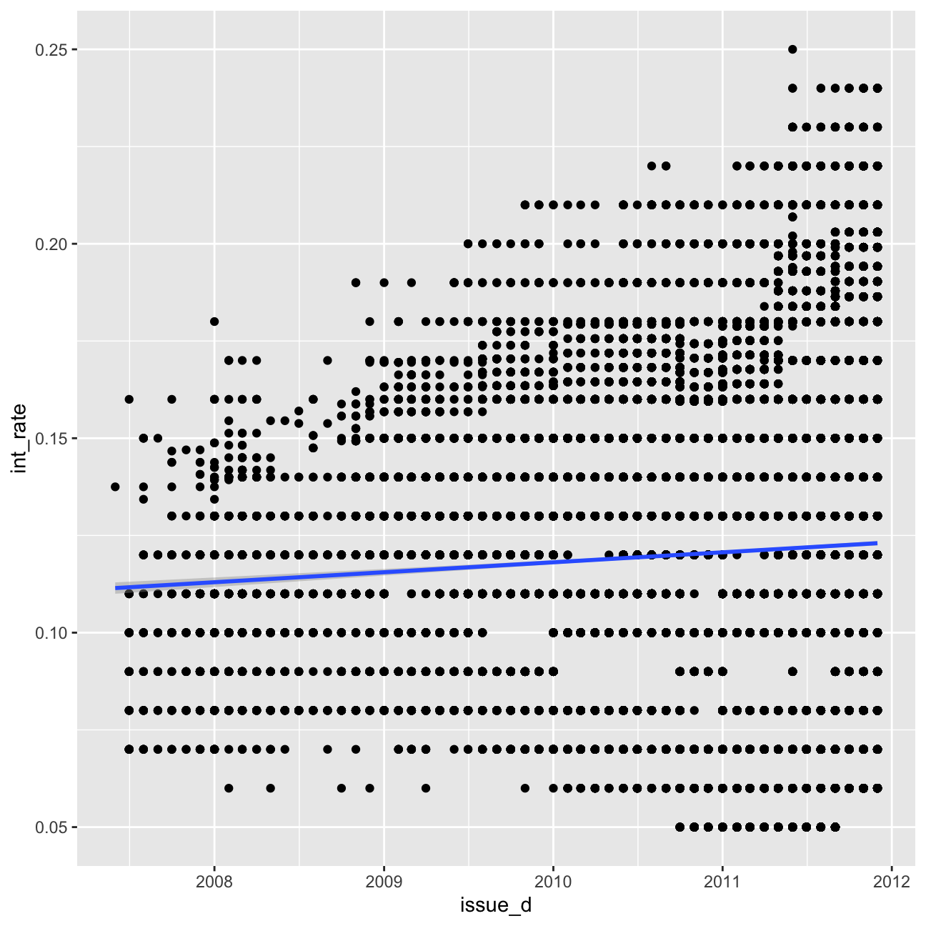

#linear time trend by grade (add code below)
ggplot(lc_clean, aes(x=issue_d,y=int_rate, colour=grade))+
  geom_point()+
  geom_smooth(method="lm")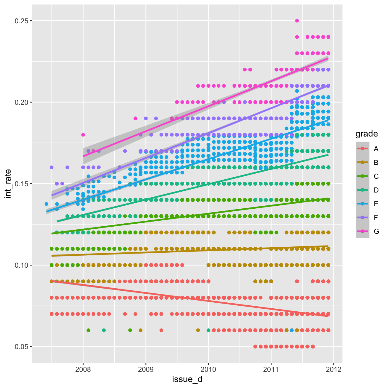

glimpse(lc_clean2)

## Rows: 37,869
## Columns: 21
## $ int_rate             <dbl> 0.05, 0.05, 0.05, 0.05, 0.05, 0.05, 0.05, 0.05, …
## $ loan_amnt            <dbl> 8000, 6000, 6500, 8000, 5500, 6000, 10200, 15000…
## $ dti                  <dbl> 2.11, 5.73, 17.68, 22.71, 5.75, 21.92, 18.62, 9.…
## $ delinq_2yrs          <fct> 0, 0, 0, 0, 0, 0, 0, 0, 0, 0, 0, 0, 0, 0, 0, 0, …
## $ annual_inc           <dbl> 50000, 52800, 35352, 79200, 240000, 89000, 11000…
## $ grade                <chr> "A", "A", "A", "A", "A", "A", "A", "A", "A", "A"…
## $ emp_length           <fct> 5 years, < 1 year, n/a, n/a, 10+ years, 2 years,…
## $ home_ownership       <chr> "MORTGAGE", "MORTGAGE", "MORTGAGE", "MORTGAGE", …
## $ verification_status  <chr> "Verified", "Source Verified", "Not Verified", "…
## $ issue_d              <date> 2011-09-01, 2011-09-01, 2011-09-01, 2011-09-01,…
## $ zip_code             <chr> "977xx", "228xx", "864xx", "322xx", "278xx", "76…
## $ addr_state           <chr> "OR", "VA", "AZ", "FL", "NC", "TX", "CT", "WA", …
## $ loan_status          <chr> "Fully Paid", "Charged Off", "Fully Paid", "Full…
## $ desc                 <chr> "Borrower added on 09/08/11 > Consolidating debt…
## $ purpose              <chr> "debt_consolidation", "vacation", "credit_card",…
## $ title                <chr> "Credit Card Payoff $8K", "bad choice", "Credit …
## $ term                 <fct> 36, 36, 36, 36, 36, 36, 36, 36, 36, 36, 36, 36, …
## $ term_months          <dbl> 36, 36, 36, 36, 36, 36, 36, 36, 36, 36, 36, 36, …
## $ installment          <dbl> 241.3, 181.0, 196.0, 241.3, 165.9, 181.0, 307.6,…
## $ emp_title            <chr> NA, "coral graphics", NA, "Honeywell", "O T Plus…
## $ quartiles_annual_inc <fct> 2, 2, 1, 3, 4, 4, 4, 4, 2, 2, 4, 3, 3, 2, 1, 3, …

#Train models using OLS regression and k-fold cross-validation
#The first model has some explanatory variables and a linear time trend

time1<-train(
  int_rate ~ loan_amnt*grade+ term+ dti + issue_d,#fill your variables here "+ issue_d"
  lc_clean,
  method = "lm",
  trControl = control)

## + Fold01: intercept=TRUE 
## - Fold01: intercept=TRUE 
## + Fold02: intercept=TRUE 
## - Fold02: intercept=TRUE 
## + Fold03: intercept=TRUE 
## - Fold03: intercept=TRUE 
## + Fold04: intercept=TRUE 
## - Fold04: intercept=TRUE 
## + Fold05: intercept=TRUE 
## - Fold05: intercept=TRUE 
## + Fold06: intercept=TRUE 
## - Fold06: intercept=TRUE 
## + Fold07: intercept=TRUE 
## - Fold07: intercept=TRUE 
## + Fold08: intercept=TRUE 
## - Fold08: intercept=TRUE 
## + Fold09: intercept=TRUE 
## - Fold09: intercept=TRUE 
## + Fold10: intercept=TRUE 
## - Fold10: intercept=TRUE 
## Aggregating results
## Fitting final model on full training set

#summary(time1) # seems like dti is corrolated with issue_d (maybe lots of people defaulted because of the crisis)

#The second model has a different linear time trend for each grade class
time2<-train(
    int_rate ~ loan_amnt*grade+ term+ dti + issue_d*grade, #fill your variables here 
    lc_clean,
   method = "lm",
    trControl = control
   )

## + Fold01: intercept=TRUE 
## - Fold01: intercept=TRUE 
## + Fold02: intercept=TRUE 
## - Fold02: intercept=TRUE 
## + Fold03: intercept=TRUE 
## - Fold03: intercept=TRUE 
## + Fold04: intercept=TRUE 
## - Fold04: intercept=TRUE 
## + Fold05: intercept=TRUE 
## - Fold05: intercept=TRUE 
## + Fold06: intercept=TRUE 
## - Fold06: intercept=TRUE 
## + Fold07: intercept=TRUE 
## - Fold07: intercept=TRUE 
## + Fold08: intercept=TRUE 
## - Fold08: intercept=TRUE 
## + Fold09: intercept=TRUE 
## - Fold09: intercept=TRUE 
## + Fold10: intercept=TRUE 
## - Fold10: intercept=TRUE 
## Aggregating results
## Fitting final model on full training set

#summary(time2)

#Change the time trend to a quarter dummy variables.
#zoo::as.yearqrt() creates quarter dummies 
lc_clean_quarter<-lc_clean %>%
  mutate(yq = as.factor(as.yearqtr(lc_clean$issue_d, format = "%Y-%m-%d")))



time3<-train(
    int_rate ~loan_amnt*grade+ term+ dti + yq ,#fill your variables here 
    lc_clean_quarter,
     method = "lm",
    trControl = control
   )

## + Fold01: intercept=TRUE 
## - Fold01: intercept=TRUE 
## + Fold02: intercept=TRUE 
## - Fold02: intercept=TRUE 
## + Fold03: intercept=TRUE 
## - Fold03: intercept=TRUE 
## + Fold04: intercept=TRUE 
## - Fold04: intercept=TRUE 
## + Fold05: intercept=TRUE 
## - Fold05: intercept=TRUE 
## + Fold06: intercept=TRUE 
## - Fold06: intercept=TRUE 
## + Fold07: intercept=TRUE 
## - Fold07: intercept=TRUE 
## + Fold08: intercept=TRUE 
## - Fold08: intercept=TRUE 
## + Fold09: intercept=TRUE 
## - Fold09: intercept=TRUE 
## + Fold10: intercept=TRUE 
## - Fold10: intercept=TRUE 
## Aggregating results
## Fitting final model on full training set

#summary(time3)

#specify one quarter dummy variable for each grade. This is going to be a large model as there are 19 quarters x 7 grades = 133 quarter-grade dummies.
time4<-train(
    int_rate ~loan_amnt*grade+ term+ dti + yq*grade ,#fill your variables here 
    lc_clean_quarter,
     method = "lm",
    trControl = control
   )

## + Fold01: intercept=TRUE 
## - Fold01: intercept=TRUE 
## + Fold02: intercept=TRUE 
## - Fold02: intercept=TRUE 
## + Fold03: intercept=TRUE 
## - Fold03: intercept=TRUE 
## + Fold04: intercept=TRUE 
## - Fold04: intercept=TRUE 
## + Fold05: intercept=TRUE 
## - Fold05: intercept=TRUE 
## + Fold06: intercept=TRUE 
## - Fold06: intercept=TRUE 
## + Fold07: intercept=TRUE 
## - Fold07: intercept=TRUE 
## + Fold08: intercept=TRUE 
## - Fold08: intercept=TRUE 
## + Fold09: intercept=TRUE 
## - Fold09: intercept=TRUE 
## + Fold10: intercept=TRUE 
## - Fold10: intercept=TRUE 
## Aggregating results
## Fitting final model on full training set

#summary(time4)

data.frame(
  time1$results$RMSE,
  time2$results$RMSE,
  time3$results$RMSE,
  time4$results$RMSE)

time1.results.RMSE	time2.results.RMSE	time3.results.RMSE	time4.results.RMSE
0.0103	0.00905	0.00908	0.00758

Based on my model, there is the evidence to suggest that interest rate change over time is significant. Including time trends or quarter dummies does improve the predictions.

Using Bond Yields

One concern with using time trends for forecasting is that in order to make predictions for future loans we will need to project trends to the future. This is an extrapolation that may not be reasonable, especially if macroeconomic conditions in the future change. Furthermore, if we are using quarter dummies, it is not even possible to estimate the coefficient of these dummy variables for future quarters.

Instead, perhaps it’s better to find the reasons as to why different periods are different from one another. The csv file “MonthBondYields.csv” contains information on the yield of US Treasuries on the first day of each month. I will you it to see if I can improve my predictions without using time dummies?.

#load the data to memory as a dataframe
bond_prices<-readr::read_csv("~/Documents/LBS/Data Science/Session 03/MonthBondYields.csv")

#make the date of the bond file comparable to the lending club dataset
#for some regional date/number (locale) settings this may not work. If it does try running the following line of code in the Console
#Sys.setlocale("LC_TIME","English")
bond_prices <- bond_prices %>%
  mutate(Date2=as.Date(paste("01",Date,sep="-"),"%d-%b-%y")) %>%
  select(-starts_with("X"))

#let's see what happened to bond yields over time. Lower bond yields mean the cost of borrowing has gone down.

bond_prices %>%
  ggplot(aes(x=Date2, y=Price))+geom_point(size=0.1, alpha=0.5)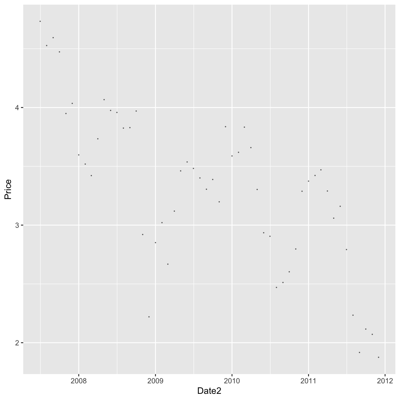

#join the data using a left join
lc_with_bonds<-lc_clean %>%
  left_join(bond_prices, by = c("issue_d" = "Date2")) %>%
  arrange(issue_d) %>%
  filter(!is.na(Price)) #drop any observations where there re no bond prices available

# investigate graphically if there is a relationship 
lc_with_bonds%>%
  ggplot(aes(x=int_rate, y=Price))+geom_point(size=0.1, alpha=0.5)+geom_smooth(method="lm")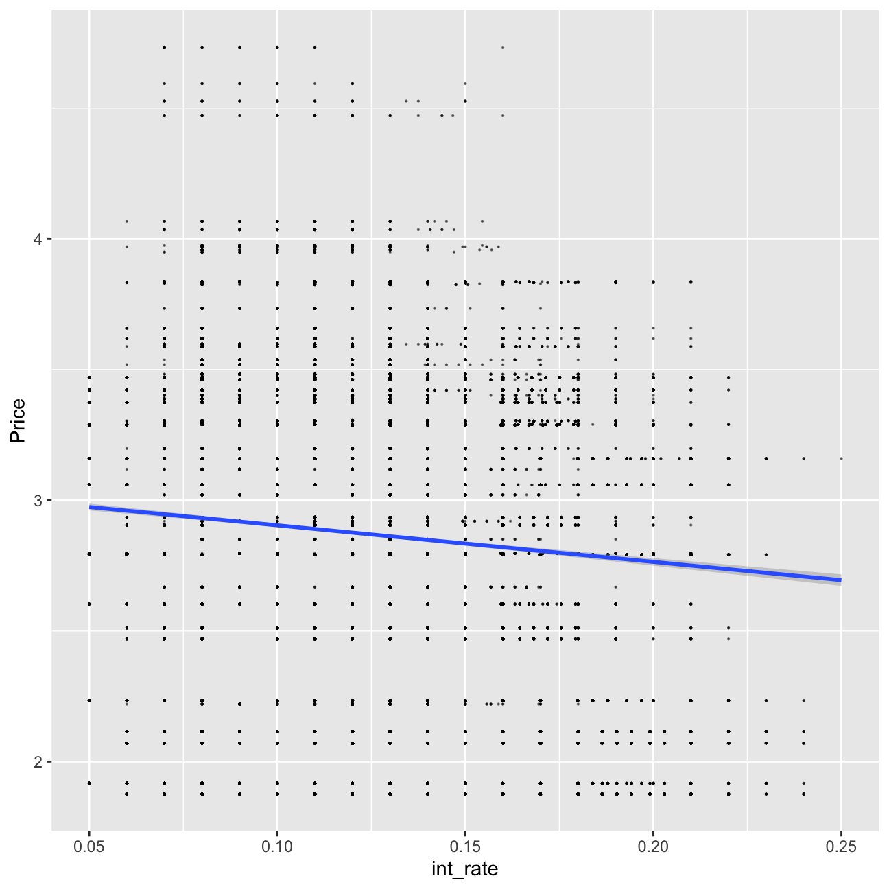

lc_with_bonds%>%
  ggplot(aes(x=int_rate, y=Price, color=grade))+geom_point(size=0.1, alpha=0.5)+geom_smooth(method="lm")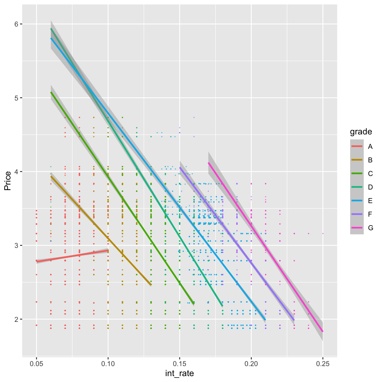

#let's train a model using the bond information


plsFit<-train(
    int_rate ~loan_amnt*grade+ term+ dti + Price*grade , #fill your variables here 
    lc_with_bonds,
   method = "lm",
    trControl = control
   )

## + Fold01: intercept=TRUE 
## - Fold01: intercept=TRUE 
## + Fold02: intercept=TRUE 
## - Fold02: intercept=TRUE 
## + Fold03: intercept=TRUE 
## - Fold03: intercept=TRUE 
## + Fold04: intercept=TRUE 
## - Fold04: intercept=TRUE 
## + Fold05: intercept=TRUE 
## - Fold05: intercept=TRUE 
## + Fold06: intercept=TRUE 
## - Fold06: intercept=TRUE 
## + Fold07: intercept=TRUE 
## - Fold07: intercept=TRUE 
## + Fold08: intercept=TRUE 
## - Fold08: intercept=TRUE 
## + Fold09: intercept=TRUE 
## - Fold09: intercept=TRUE 
## + Fold10: intercept=TRUE 
## - Fold10: intercept=TRUE 
## Aggregating results
## Fitting final model on full training set

summary(plsFit)

## 
## Call:
## lm(formula = .outcome ~ ., data = dat)
## 
## Residuals:
##      Min       1Q   Median       3Q      Max 
## -0.11745 -0.00581 -0.00030  0.00649  0.04073 
## 
## Coefficients:
##                     Estimate Std. Error t value Pr(>|t|)    
## (Intercept)         6.79e-02   5.36e-04  126.68  < 2e-16 ***
## loan_amnt           1.80e-07   1.86e-08    9.64  < 2e-16 ***
## gradeB              5.35e-02   6.99e-04   76.54  < 2e-16 ***
## gradeC              8.63e-02   7.84e-04  110.05  < 2e-16 ***
## gradeD              1.19e-01   8.94e-04  133.27  < 2e-16 ***
## gradeE              1.43e-01   1.17e-03  122.79  < 2e-16 ***
## gradeF              1.67e-01   1.79e-03   93.10  < 2e-16 ***
## gradeG              1.90e-01   3.46e-03   55.06  < 2e-16 ***
## term60              1.51e-03   1.32e-04   11.38  < 2e-16 ***
## dti                 2.80e-05   7.45e-06    3.76  0.00017 ***
## Price               1.30e-03   1.63e-04    8.01  1.2e-15 ***
## `loan_amnt:gradeB` -9.48e-08   2.25e-08   -4.21  2.5e-05 ***
## `loan_amnt:gradeC` -2.20e-07   2.42e-08   -9.09  < 2e-16 ***
## `loan_amnt:gradeD` -1.99e-09   2.57e-08   -0.08  0.93842    
## `loan_amnt:gradeE`  6.44e-08   2.79e-08    2.31  0.02083 *  
## `loan_amnt:gradeF`  6.99e-08   3.84e-08    1.82  0.06869 .  
## `loan_amnt:gradeG` -1.21e-07   6.77e-08   -1.78  0.07491 .  
## `gradeB:Price`     -5.77e-03   2.18e-04  -26.47  < 2e-16 ***
## `gradeC:Price`     -8.00e-03   2.43e-04  -32.93  < 2e-16 ***
## `gradeD:Price`     -1.27e-02   2.79e-04  -45.59  < 2e-16 ***
## `gradeE:Price`     -1.53e-02   3.61e-04  -42.29  < 2e-16 ***
## `gradeF:Price`     -1.67e-02   5.36e-04  -31.10  < 2e-16 ***
## `gradeG:Price`     -1.78e-02   9.98e-04  -17.83  < 2e-16 ***
## ---
## Signif. codes:  0 '***' 0.001 '**' 0.01 '*' 0.05 '.' 0.1 ' ' 1
## 
## Residual standard error: 0.00958 on 37845 degrees of freedom
## Multiple R-squared:  0.934,  Adjusted R-squared:  0.934 
## F-statistic: 2.43e+04 on 22 and 37845 DF,  p-value: <2e-16

From the above, after including in my model “Price”, I can infer that the bonds have the explanatory power. However, the explanatory power increases the Adjusted R-squared less than the time trend/quarter variables.

Further improvement

My final model can be observed below. It has an explanatory power with adjusted R-squared of 93.57%. It has a Confidence Interval at 95% of ±0.01852592%. It can be used to accurately predict the mean. I used the linear model with method of stepwise k-fold cross validation.

lc_with_yq_bonds<- lc_with_bonds %>% 
  mutate(yq = as.factor(as.yearqtr(issue_d, format = "%Y-%m-%d")))

model_wild_west <- train(
    int_rate ~loan_amnt*grade+ term+ dti + poly(Price, 3)*grade, #fill your variables here 
    lc_with_yq_bonds,
   method = "lm",
    trControl = control
   )

## + Fold01: intercept=TRUE 
## - Fold01: intercept=TRUE 
## + Fold02: intercept=TRUE 
## - Fold02: intercept=TRUE 
## + Fold03: intercept=TRUE 
## - Fold03: intercept=TRUE 
## + Fold04: intercept=TRUE 
## - Fold04: intercept=TRUE 
## + Fold05: intercept=TRUE 
## - Fold05: intercept=TRUE 
## + Fold06: intercept=TRUE 
## - Fold06: intercept=TRUE 
## + Fold07: intercept=TRUE 
## - Fold07: intercept=TRUE 
## + Fold08: intercept=TRUE 
## - Fold08: intercept=TRUE 
## + Fold09: intercept=TRUE 
## - Fold09: intercept=TRUE 
## + Fold10: intercept=TRUE 
## - Fold10: intercept=TRUE 
## Aggregating results
## Fitting final model on full training set

#summary(model_wild_west)

0.009452*1.96

## [1] 0.0185

Use of additional sources

I will now use other publicly available datasets to further improve performance (e.g., quarterly data on US inflation or CPI).

Changes in CPI should correlate to changes in inflation, therefore such a variable can better explain behaviour of interest rates in the market as behaviour of inlfation partially explaines the behaviour of loan takers and actions of investors/government.

CPI_df <- read_csv("~/Documents/LBS/Data Science/Session 03/CPALTT01USM657N.csv") %>%  clean_names() # use janitor::clean_names()

glimpse(CPI_df)

## Rows: 727
## Columns: 2
## $ date            <date> 1960-01-01, 1960-02-01, 1960-03-01, 1960-04-01, 1960…
## $ cpaltt01usm657n <dbl> -0.340, 0.341, 0.000, 0.340, 0.000, 0.339, 0.000, 0.0…

lc_with_CPI<-lc_with_bonds %>%
  left_join(CPI_df, by = c("issue_d" = "date")) %>%
  arrange(issue_d)

glimpse(lc_with_CPI)

## Rows: 37,868
## Columns: 27
## $ int_rate            <dbl> 0.07, 0.07, 0.07, 0.07, 0.07, 0.07, 0.07, 0.08, 0…
## $ loan_amnt           <dbl> 5750, 5000, 5000, 5000, 5000, 5000, 5000, 5400, 5…
## $ dti                 <dbl> 0.27, 2.55, 0.00, 3.83, 2.29, 0.31, 3.72, 3.00, 5…
## $ delinq_2yrs         <fct> 0, 0, 0, 0, 0, 0, 0, 0, 0, 0, 0, 0, 0, 2, 0, 0, 0…
## $ annual_inc          <dbl> 125000, 40000, 150000, 95000, 120000, 85000, 2000…
## $ grade               <chr> "A", "A", "A", "A", "A", "A", "A", "A", "A", "A",…
## $ emp_length          <fct> 10+ years, 6 years, 8 years, 7 years, 8 years, 1 …
## $ home_ownership      <chr> "MORTGAGE", "RENT", "MORTGAGE", "MORTGAGE", "MORT…
## $ verification_status <chr> "Not Verified", "Not Verified", "Not Verified", "…
## $ issue_d             <date> 2007-07-01, 2007-07-01, 2007-07-01, 2007-07-01, …
## $ zip_code            <chr> "020xx", "547xx", "303xx", "017xx", "017xx", "537…
## $ addr_state          <chr> "MA", "WI", "GA", "MA", "MA", "WI", "MD", "GA", "…
## $ loan_status         <chr> "Fully Paid", "Fully Paid", "Fully Paid", "Fully …
## $ desc                <chr> "consolidate debt on several credit cards.", "Hel…
## $ purpose             <chr> "debt_consolidation", "car", "home_improvement", …
## $ title               <chr> "consolidate debt", "$5000 car loan to be paid ba…
## $ term                <fct> 36, 36, 36, 36, 36, 36, 36, 36, 36, 36, 36, 36, 3…
## $ term_months         <dbl> 36, 36, 36, 36, 36, 36, 36, 36, 36, 36, 36, 36, 3…
## $ installment         <dbl> 178.7, 155.4, 155.4, 155.4, 155.4, 155.4, 155.4, …
## $ emp_title           <chr> "FDA", "Norman G. Olson Insurance", "Oracle Corpo…
## $ Date                <chr> "Jul-07", "Jul-07", "Jul-07", "Jul-07", "Jul-07",…
## $ Price               <dbl> 4.73, 4.73, 4.73, 4.73, 4.73, 4.73, 4.73, 4.73, 4…
## $ Open                <dbl> 4.73, 4.73, 4.73, 4.73, 4.73, 4.73, 4.73, 4.73, 4…
## $ High                <dbl> 4.73, 4.73, 4.73, 4.73, 4.73, 4.73, 4.73, 4.73, 4…
## $ Low                 <dbl> 4.73, 4.73, 4.73, 4.73, 4.73, 4.73, 4.73, 4.73, 4…
## $ `Change %`          <chr> "-5.85%", "-5.85%", "-5.85%", "-5.85%", "-5.85%",…
## $ cpaltt01usm657n     <dbl> -0.0254, -0.0254, -0.0254, -0.0254, -0.0254, -0.0…

model_wild_west2 <- train(
    int_rate ~loan_amnt*grade+ term+ dti + poly(Price, 3)*grade+cpaltt01usm657n*grade , #fill your variables here 
    lc_with_CPI,
   method = "lm",
    trControl = control
   )

## + Fold01: intercept=TRUE 
## - Fold01: intercept=TRUE 
## + Fold02: intercept=TRUE 
## - Fold02: intercept=TRUE 
## + Fold03: intercept=TRUE 
## - Fold03: intercept=TRUE 
## + Fold04: intercept=TRUE 
## - Fold04: intercept=TRUE 
## + Fold05: intercept=TRUE 
## - Fold05: intercept=TRUE 
## + Fold06: intercept=TRUE 
## - Fold06: intercept=TRUE 
## + Fold07: intercept=TRUE 
## - Fold07: intercept=TRUE 
## + Fold08: intercept=TRUE 
## - Fold08: intercept=TRUE 
## + Fold09: intercept=TRUE 
## - Fold09: intercept=TRUE 
## + Fold10: intercept=TRUE 
## - Fold10: intercept=TRUE 
## Aggregating results
## Fitting final model on full training set

#summary(model_wild_west2)

Next Project

Predicting interest rates using K-fold CV,LASSO & OLS regression

Load and prepare the data

ICE the data: Inspect, Clean, Explore

Explore the data by building some visualizations.

Estimatimation of simple linear regression models

Questions on the model

Feature Engineering

Conclusions

Out of sample testing

k-fold cross validation

Conclusions

Sample size estimation and learning curves

Regularization using LASSO regression

LASSO compared to OLS

Using Time Information

Using Bond Yields

Further improvement

Use of additional sources

Contact me